The Null Hypothesis

Null hypothesis testing is a method of assessing whether there is sufficient evidence in the data to reject the null hypothesis, thereby lending support to an alternative theory or claim.

The alternative theory is what we are trying to gather evidence for. This test does not provide absolute truths or exact probabilities that a hypothesis is true, but instead evaluates whether the observed data are statistically significant enough to suggest that a property or effect may exist.

Note: This article has been designed for the context of financial trading.

Stage 1: Defining the hypotheses

The first step is to take the initial idea or claim and break it down into two clearly defined theories or definitions, referred to as hypotheses.

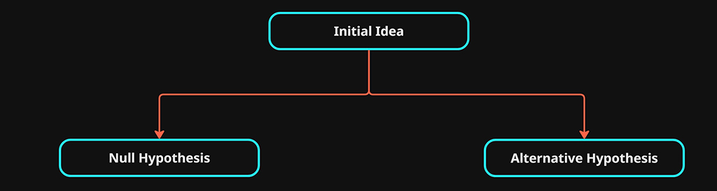
The two theories need to oppose each other. One of the theories has an effect or property that we are trying to find evidence for. This will be referred to as the alternative hypothesis $H_1$ and the other theory assumes there is no difference or effect, this is our null hypothesis $H_0$.

$$ H_0 \ vs.\ H_1 $$

Null hypothesis $H_0$: This is the theory that states the effect does not exist.

“Trading signal X has no significant benefit on Y”
Alternative hypothesis $H_1$: This is the theory we are trying to test, that suggests an effect or property may exist.

“Trading signal X does have a significant benefit on Y”

Note: “signal X” will be used a placeholder. “Y” is also a placeholder

From a top level perspective these definitions are clear but they are not very actionable. We need to give more detail into how each theory can be defined.

If $H_1$ suggests that trading signal X is effective, Then $H_0$ needs to represent the opposite of an effective trading signal, One way to model this could be to compare the results of $H_1$ to the results of a randomly generated trading signal.

The improved definitions would now define as follows:

Null hypothesis $H_0$: Trading signal X has no significant benefit over a random trading signal.

$H_0$ represents random trading signals

Alternative hypothesis $H_1$: Trading signal X does have a significant benefit over a random trading signal.

$H_1$ represents signal X trading signals

2nd Stage: Data Generation

Now we have clearly defined hypotheses, we need a method of generating and collecting data that will be used for our test. The methods can vary depending on what is being tested. In our case, we will be using automated backtesting to generate and gather the necessary data.

For each hypothesis $H_0$ & $H_1$, data will need to be generated separately. These two sets of data will be compared to one another in order to establish if $H_1$ has statistical significance.

$H_0$: Backtest from a trading system that uses a randomly generated entry signal.
$H_1$: Backtest from a trading system that uses signal X as entry signals.

Each set of backtests should be carried out with exactly the same trade logic and setup factors, with the exception of the property or effect you are testing. In this case the only differences between the tests will be the trade entry logic.

The alternative hypothesis $H_1$ data will generated with a standard backtest that has the entry signal logic defined by “signal X”. The data that will be collected from this backtest is a single metric or statistic, referred to as the test statistic. More on this to come.

The null hypothesis $H_0$ data will be achieved with the following additional steps.

Monte Carlo Simulation

To approximate the data required for the null hypothesis, we will be using Monte Carlo simulations to introduce random sampling into our backtesting results.

First we need to adapt the backtest that was used for $H_1$. The only difference should be the trading entry signal logic. We will be replacing the entry signal logic of “Signal X” with a randomly generated signal that determines when to enter trades.

Unlike the data for $H_1$, which comes from a single backtest, the data for $H_0$ will need to be represented as a distribution of many backtest results.

Ideally we need to be generating anywhere between 1,000 to 10,000 individual backtests to represent the null hypothesis.

This will be referred as the Null Distribution. A collection of 1000’s of backtest results.

Each back test will have the same logic, a randomly generated entry signal. The only difference between the backtests will be the random seed value used to calculate the entries for each trade. As a result each version of the backtest will have trades with different entry times.

This gives us a large enough distribution or spread of results to represent the possible outcomes more accurately (law of large numbers). If we just did a single backtest, this would only provide a single outcome, we need a large range in order to represent the possibilities of randomness more accurately.

For each iteration of backtest, A single metric will be collected. This needs to be the same type of metric that was collected from the $H_1$ backtest (test statistic).

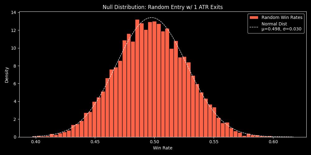
Below is an example of a null distribution , it represents the win rate(test statistic) of 10,000 backtests that use random timing for trade entries.

You can see that the results vary from a win rate of 0.4 to 0.6. If we just had a single backtest with random entries, we would not have an understanding of the entire range that are plausible while using random entries.

Test Statistic (Observed Statistic)

In order to compared the data sets of $H_0$ & $H_1$. We need a type of measurement that can be used to compare both sets of data. This metric is either referred to as the observed statistic or the test statistic.

The metric selected needs to embody the effect or property that is being tested. The effect needs to be observable from this metric alone.

Examples of this metric may be the win rate or sharpe ratio.

The definition of $H_1$ is only concerned with testing the quality of the signal X as a trade entry strategy. That quality is measured by its probability over random.

Because we are strictly testing for the forecasting ability of signal X compared to random. We are able to configure the trade logic in the backtest setup so that by using the calculated win rate as our single metric, we are able to observe the effect from this test statistic.

Test Statistic: Win Rate

This single statistic allows us to observe the effect described by $H_1$.

Data collection outcome:

$H_1$ – The result of a conventional backtest. A single observed statistic, win rate.
$H_0$ – A collection of win rate statistics from each backtest. 1,000-10,000 individual test statistics, forming the null distribution.

NOTE: Its important to consider carefully what observed statistic is used. The test (backtest) needs to be designed in a way that the selected statistic measures what is being stated in both hypotheses.

Third Stage: Analysis

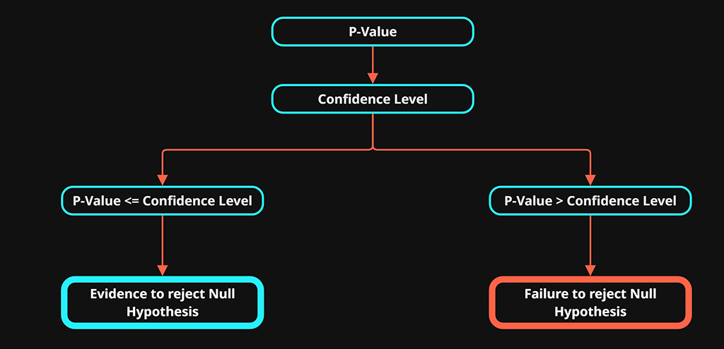
Once we have the two data sets we can use a p-value along with a confidence level to help assess our analysis.

P-Value

The p-value stands for “probability value”. It is this value that is used to assess the results of the hypothesis testing.

The p-value helps us understand whether our results would be unusual under the assumption that the null hypothesis is correct.

How likely is it that random trade entries could achieve the same or better results than those observed in our backtest using signal x

Lets look at how we calculate p-value. There are three main ways used to calculate p-value. They are selected to answer slightly different questions.

Right-tailed: Is the observed statistic significantly greater than the null expectation?
Left-tailed: Is the observed statistic significantly less than the null expectation?
Two-tailed: Is the observed statistic significantly different, in either direction?

We will be using right-tailed for our example as we are looking for significantly better-than-null performance.

$d={t_1,t_2,…,t_n}$ : Each individual test statistic from the null distribution
$t_{obs}$ : the observed test statistic from our backtest using signal x.
$n$: The total number of test statistics in the null distribution

right-tailed p-value:

$$ p = \frac{1}{n} \sum_{i=1}^n 1(t_i \ge t_{obs}) $$

In simple terms, for every data point in the null distribution, we check if it is greater than or equal to our observed test statistic.

We then sum these comparisons to calculate the probability, which is the p-value

The p-value is a number between 0 and 1, describing the probability of observing data as extreme as what we saw, assuming the null distribution is correct.

To determine if the p-value is significant, we compare it to a threshold. We will use example thresholds below for demonstration

A p-value that is $\le 0.05$

The observed results is unlikely under $H_0$.
This is evidence against $H_0$ and in turn evidence for $H_1$
Let’s say the p-value is 0.05. This means there is a 5% chance of seeing results as extreme as ours purely by random chance if the null hypothesis were true
Significant evidence to reject $H_0$ -> Statistical evidence in favour of the alt $H_1$.

A p-value that is $\gt 0.05$

The observed results are likely under $H_0$
This is evidence against $H_1$ and in turn evidence for $H_0$
Let’s say the p-value is 0.10. This means there is a 10% chance of seeing results as extreme as ours purely by random chance if the null hypothesis were true.
Failure to reject $H_0$ -> No statistical evidence in favour of the alt $H_1$.

In simple terms:

The smaller the p-value, the less likely the results can be observed by random chance.

Significance Level $\alpha$

The threshold we choose to determine if we have enough evidence to reject $H_0$ or not, is referred to as the significance level $\alpha$.

$\alpha$ = 0.05 / 5% , this is the standard significance level.
$\alpha$ = 0.01 / 1% , this provides a stricter criterion and as a result we can have more confidence in $H_1$ if the p-value is less than or equal to this significance level.

The smaller the p-value, the less likely the observed results are due to random chance alone, providing more evidence that the effect is statistically significant.

The significance level $\alphaα$ you set determines how strict your test is. Common choices are 1% and 5%. A 10% level is sometimes used but is considered less reliable, since it allows a 10% chance of a false positive.

At a 10% significance level, there is a higher risk that the observed effect could be explained by random variation rather than a true effect.

Confidence Level:

Confidence level = 1-$\alpha$
A significance level of 0.05 (5%) is corresponding to a 95% confidence level

Quick Overview:

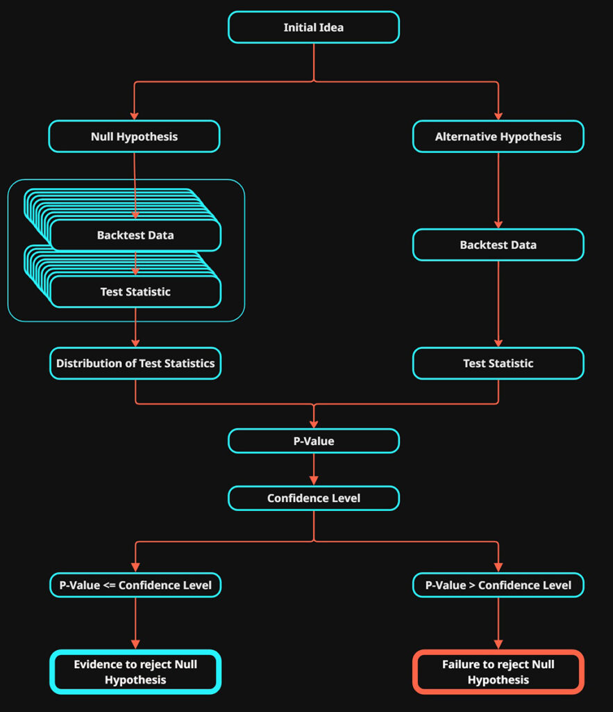
The basis steps of a hypothesis test:

1. Define The Hypotheses

Null Hypothesis $H_0$
Alternative Hypothesis $H_1$

2. Select a Test Statistic

3. Generate Data Sets:

$H_0$ perform backtests to generate a distribution of test statistics (the null distribution).
$H_1$ run a backtest to calculate the observed test statistic

4. Decide on a Significance Level (α):

This is your threshold for rejecting $H_0$.
Common choice: α = 0.05 (5%)

5. Compare p-value to α:

If p ≤ α → Reject $H_0$ (evidence in favour of alt hypothesis)
If p > α → Failure to reject $H_0$ (not enough evidence for alt hypothesis)

When to Use P-Value Testing

You want to test a specific claim or effect in a data sample.
You have enough data to make probabilistic conclusions.
You want to make objective, data-driven decisions.
You are comparing two or more groups, and want to know if differences are real or due to chance.

Limitations

1. Misinterpretation of the P-Value

P-value ≠ probability the null hypothesis is true or false.
It’s about the probability of $H_1$ occurring in the data of $H_0$.
It answers how common or unlikely is (\H_1\) to occur in (\H_0\).

2. Statistical Significance ≠ Practical Significance

A result may be “statistically significant” but have tiny or meaningless real-world impact.
E.g., a drug improves recovery by 0.1% with p=0.01. Is it worth it?

3. P-Hacking / Multiple Testing

If you run lots of tests, some will come up significant just by chance.
This inflates false positives unless you correct for it (e.g., Bonferroni correction).

4. Overreliance on Arbitrary Thresholds

People treat 0.05 like a sacred cut off, but it’s just a convention.
P=0.049 → “Significant!” vs. P=0.051 → “Not significant!” is a silly binary.

5. Small Sample Sizes

With too little data, you might miss real effects (false negatives).
With too much data, even tiny effects become “significant”.

How Effective Is It

Strengths

Well-established and widely used in scientific and business research.
Offers a clear framework for testing assumptions.
Works well when the assumptions (normality, independence, etc.) hold.

Weaknesses

Easy to misuse or misinterpret.
Can be gamed (e.g., by cherry-picking results).
Doesn’t provide the size or direction of an effect (you need confidence intervals or effect sizes for that).