

Introduction
In an effort to get back into financial trading as a hobby, The most logical option for my personality type is algorithmic aka quant trading. This bears two main advantages. The first being I don’t have to spend hours staring at charts and the second but probably most important, Is it allows me to be able to test trading ideas out for statistical significance prior to actually trading those ideas. Manual back-testing offers some form of statistical testing but its very labour intensive and can be more prone to errors.
In order for me to have any confidence in a trading strategy, I need a robust framework that allows me to rigorously test out ideas prior to spending time and money putting them to the test in the market.
The Framework
Below is the breakdown of the what this framework tests for, some of the tests are essential while others are optional depending on requirements and characteristics of the strategy.
- Null Hypothesis Test
- Statistical significance
- Additional Testing:
- Robustness
- Generalizability
Only if the null hypothesis test shows statistical significance should we continue with the additional testing.
Additional testing:
A collection of additional tests, not all are necessarily needed however some of the additional tests should be carried out prior to trading live.
Null Hypothesis Testing
Testing for: Statistical significance
Read The Null Hypothesis for more detail null hypothesis testing.
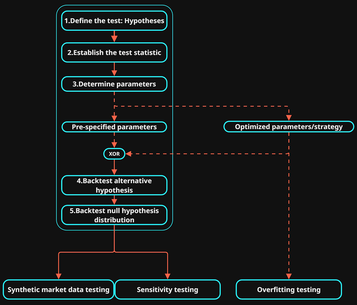
Steps 1-6 relates to null hypothesis testing.
1.Define The Test: Hypotheses
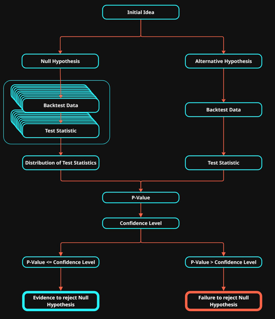
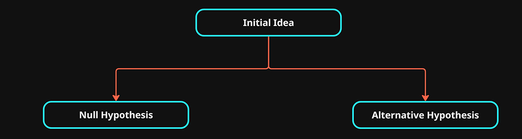
We must clearly define what we’re testing for, as simply as possible. This becomes the alternative hypothesis \(H_1\)
We then must clearly define what a test would be that provides evidence against \(H_1\), This is our null hypothesis \(H_0\).
The null hypothesis assumes there is no benefit to the strategy, while the alternative hypothesis is the claim we want to find evidence to support.
We are testing to see if the alternative hypothesis is statistically significant against the null hypothesis.
$$ H_1 > H_0 $$
OUTPUT: An exact definition of how the theory is being tested and how it can be disproved.
2.Establish The Observed Statistic
In order to compare between the two hypothesis tests \(H_0 \ \& \ H_1\). We must have a clear metric that determines if \(H_1\) has statistical significance or not. The metric should be as simple as possible and objectively determines what the alternative hypothesis is theorizing.
OUTPUT: The selected statistic / metric that measures the theory that is being proposed by \(H_1\)
Test statistic and observed statistic are used interchangeably.
3.Determine The Parameter Values
A parameter is any value we can tweak to adjust the outcome of the strategy.
This can be approached in 1 of 2 ways:
- Pre-specified: This is when we start with parameter values that are “hard-coded” from the start, based on either theory, market intuition or common convention. Pre-specifying parameters values is the most robust as it protects against any overfitting that may occur to your system.
- Optimized: Sometimes referred to as P-hacking, when any adjustable parameter of the setup is adjusted after observing the outcome. This can be achieved with data-mining or running multiple backtests with different parameter values and selecting the optimum configuration. This can lead to overfitting to the test data and additional testing is required to ensure generalization.
OUTPUT: Pre-specified parameter values or if optimized parameter values will be used, possibly a range of values to test.
4.\(H_1\) Backtest: Alternative Hypothesis
The alternative hypothesis \(H_1\) is the test we are hoping to either find evidence for or against.
This is our theory that will be tested via a backtest on real market data.
Its vital that this test is carried out with the exact same mechanics and logic that will be traded if decided to carry through to live trading.
The following aspects that need to be maintained and executed identically in both null hypothesis testing \(H_0\) and the alternative hypothesis testing (\H_1\).
- Market Data
- Number of trades executed
- Testing Statistic (observed)
- Trading Mechanics / Strategy
- The only exception should be the logic that is used to establish the aim of the null hypothesis or the alt hypothesis.
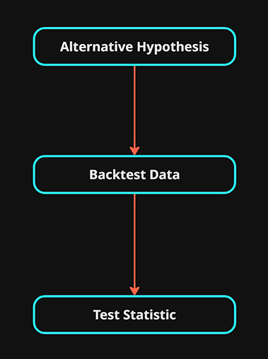
OUTPUT: The resulting test statistic that was selected previously. This statistic is calculated from the results of the backtest. i.e “win rate” ,”expectant value” or even “PnL”.
Also referred to as the observed statistic.
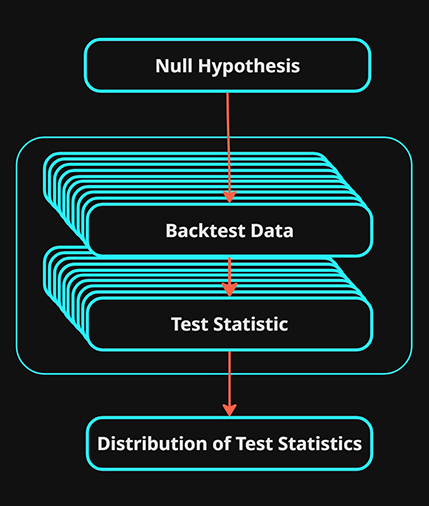
5.\(H_0\) Backtest: Null Hypothesis Distribution
The null hypothesis \(H_0\) is the baseline that does not contain the effect described in \(H_1\), if we are testing a trading strategy entry signal , we often would want to ensure that this entry signal provides better results than random.
We want to generate a distribution of backtests that will be used to compare \(H_1\) against.
Using the random entry signal as an example, instead of generating a single backtest that uses random entry signals as the trading signal. We would generate 10,000 backtests that each produce the same test statistic, the collection of test statistics from the 10,000 backtests would be collated together in a distribution that we can compare the test statistic from \(H_1\) against.
In order for the backtests generated at this stage to be the most accurate we need to ensure that we match as many of the same conditions used in the \(H_1\) backtest as possible:
- Market Data
- Number of trades executed
- Testing Statistic Type
- Trading Mechanics / Strategy
- The only exception should be the logic that is used to establish the aim of the null hypothesis.
OUTPUT: A distribution of test statistics from multiple backtests that adhere to the criteria of \(H_0\)
6.Evaluation
Up until this point we have generated two sets of data. The single test statistic that has been generated from the \(H_1\) backtest and the distribution of test statistics that have been gathered from the multiple backtests carried out under \(H_0\).
Below is an example, the histogram represents the null hypothesis distribution of test statistics , in this case it is win rate. The cyan line represents the test statistic for \(H_1\) within distribution of test statistic for \(H_0\).
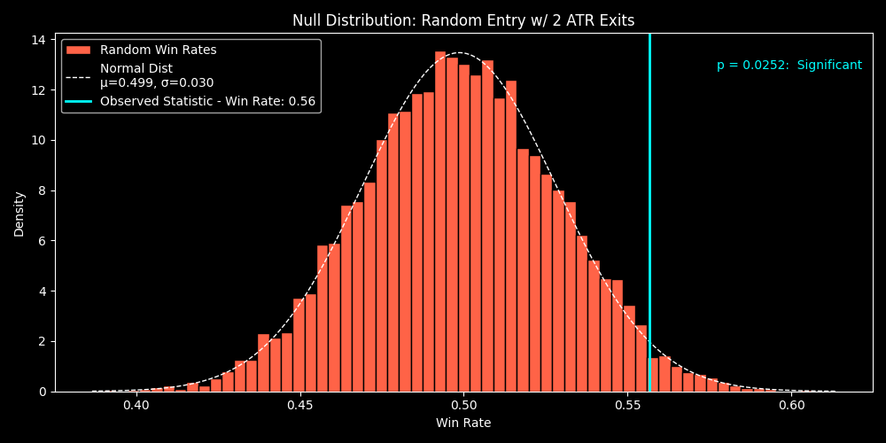
Intuitively, we can see that the test statistic from the alt hypothesis backtest is better than the majority of the null hypothesis tests. However the same results for the test statistic do still occur in the null hypothesis testing. The small tail on the right contains results that are either the same or better than the result from the alt hypothesis test.
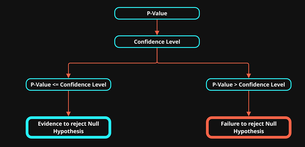
Using these two data sets we will calculate a P-value that represents the probability of \(H_1\) occurring in the distribution of \(H_0\) results. Our decision will be made based on the P-value relative to the significance level \(\alpha\)
This will help us understand how likely the desired results are to occur randomly.
Based on the result from this test, we can either conclude that we have statistical evidence to reject the null hypotheses or failure to reject the null hypotheses.
- P-value \(\le \alpha\): Evidence to reject the null hypothesis. Test was successful, proceed with further testing if required.
- P-value \(> \alpha\): Failure to reject the null hypothesis. Consider discontinuing or re-evaluating the testing strategy.
Read The Null Hypothesis for more detail null hypothesis testing.
Additional Tests
This section contains a collection of testing concepts that help to validate a trading strategy further.
Prior to taking a trading strategy live, it is recommended that the following analysis has been carried out.
- Walk-forward testing (out-of-sample)
- Market regime testing
- This can be covered by the out-of-sample testing depending on the market data used
- Operational cost simulation
Optionally, parameter sweep test and synthetic market data testing can also be used if required.
The following tests fall into two categories:
- Robustness: Testing for resistance to any reasonable change, whether to internal logic or reasonable change to input data.
- parameter tweaks
- changes in operational costs
- changes in data granularity
- moderate changes in volatility regimes
- Generalisation: Testing the strategy’s performance on unseen real market data.
- New price data
- New market conditions
A strategy that does not perform well under these variations may be weak in design or overfitted due to excessive optimization and will likely not perform well in real market conditions.
Walk-forward Analysis
Testing for: Generalization
Walk-forward analysis is considered the most realistic out-of-sample test when needing to optimize a strategy and minimize overfitting.
The historical data needs to be split into chunks, where the testing and optimization is carried out on the first in-sample data chunk, then tested on the next out-of-sample data chunk, then refined on the next in-sample data data and so on and so forth.

The backtesting results from the out-of-sample historical data becomes the result from this analysis. If it performs well in the out-of-sample chunk then its a good sign that the strategy has not been overfit.
Market Regime Testing
Testing for: Robustness
A regime is determine by the market conditions found in data.
Prior to taking a strategy live, its recommended to test the strategy in historical data that contains a range of different regimes in order to help ensure the strategy is robust enough to perform in multiple market conditions.
Market Segmentation:
- Segment historical data by regime: bull, bear, sideways, volatility levels etc — and test strategy performance in each.
- Evaluate whether strategy performs only in specific conditions.
Note: This can be carried out at the same time as the walk-forward analysis if the historic data used contains the correct variation in market regimes
Operational Cost Simulation
Testing for: Robustness
Trading is subjected to multiple direct and indirect costs such as the fees, spread and slippage.
Prior to taking a strategy live, its recommended to test the strategy under realistic simulated trading conditions that emulate the operation costs.
- Run the strategy under a range of operational cost scenarios to ensure its robust to varying costs and the possible extremes.
Parameter Sweep (Grid Search)
Testing for: Robustness
This tests how your strategy performs as you vary its input parameters (e.g., MA lengths) across a wide range of values.
This process can be used in multiple ways:
- If small changes in parameter values lead to the performance dropping dramatically, than this suggests the strategy has been overfit.
- This process can also be used to P-hack if optomizing the strategy is desired, however overfitting can easily occur whaen doing so.
Overfitting essentially will mean that the strategy isn’t generalized and since the market will always be different from historical data. The lack of generalization will mean it wont perform well with the slight changes that naturally occur in market conditions.
Synthetic Market Data Testing
Testing for: Robustness
Synthetic market data is taking the real market data and modifying it to create a variation of the market data that can be used for additional backtesting.
This is often referred to as bootstrapping or bootstrapped data. The specific variant that will be used in this framework is block bootstrapping.
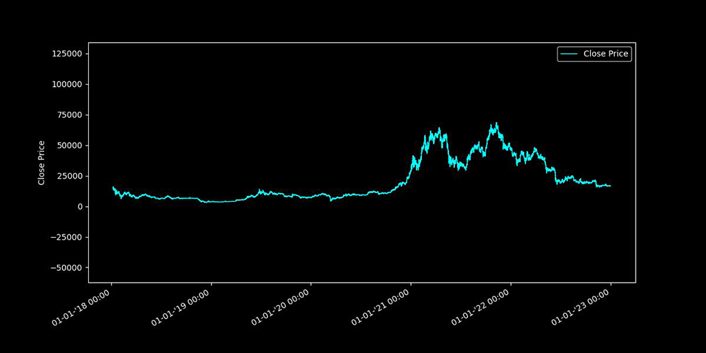
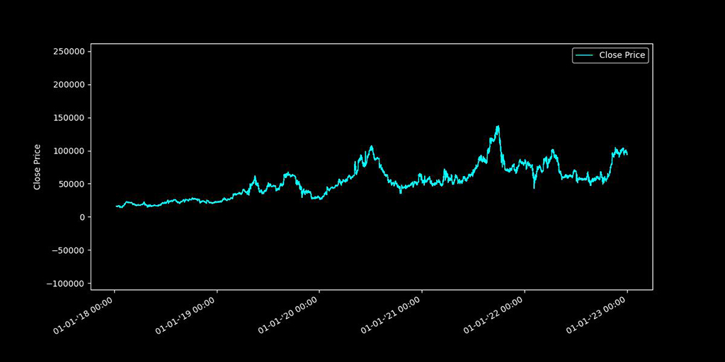
Original Data
Block Bootstrap Data
Block bootstrapping is designed to change the market structure of the data , while maintaining key statistical characteristics of the original data.
This creates a novel market data that still behaves somewhat similarly to the real market data.
The new data can effectively be used as synthetic out-of-sample data. However there is one key characteristic that is useful.
Synthetic data removes the human observation element. If the thesis of a trading strategy is dependant on the trading resulted from human observation, then in theory the same strategy should not perform well on bootstrapped data, as no one has observed it to trade.
The performance of a strategy while using bootstrapped data may depend on the nature of the strategy , the idea behind block bootstrap data is to re-sample the original market structure into something new while maintaining the other market characteristics.
if the strategy relies on the the market long term structure, such as with trend trading strategies, then the strategy should perform poorly while using this data.
Conversely if the strategy does not heavily rely on large market structures, the in theory it should still perform fairly well on the bootstrap data, Although a drop in performance is to be expected.