
Note: This study is still in progress. Consider it a rough draft. The model breakdown is still actively being blocked out.
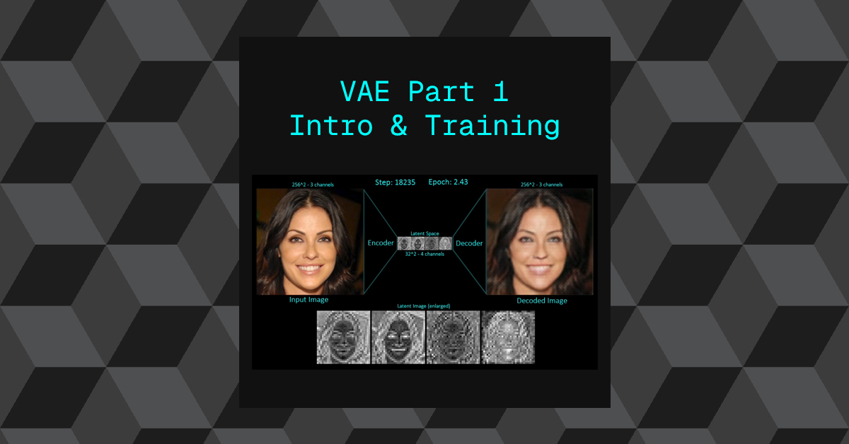
A variational autoencoder is a specific type of autoencoder that is used to convert an image from pixel space into latent space and back again.
All autoencoders are used to compress data, the variational autoencoder is used to compress down to latent space specifically.
We will be focusing on the Stable Diffusion–style VAE (LDM Autoencoder).
Citations and accreditation
Note: its worth noting that in order to help make the code more readable, I have simplified the implementation where possible and hardcoded values.
This model is a convolutional hierarchical variational autoencoder, which means it is a neural network designed to compress images and then rebuild them, using convolutional layers that are especially good at handling image data (like edges, textures, and shapes). In simple terms, it learns how to shrink an image into a smaller, more manageable internal representation, and then expand it back into an image that looks as close as possible to the original.
It is designed to compress high-resolution images into a low-dimensional spatial latent representation, which means a large image (for example, 256×256 pixels) is turned into a much smaller grid of numbers that still preserves the overall structure of the image. You can think of this latent representation as a compact “summary” of the image that keeps the important visual information while discarding unnecessary detail.
The encoder progressively downsamples the input image through residual convolutional blocks, transforming a 256×256 RGB image into a compact latent tensor while preserving semantic structure. This means the image is gradually reduced in size step by step, rather than all at once, using layers that help the network remember important features such as faces, objects, or shapes even as the resolution shrinks. The residual connections help prevent information loss and make training more stable.
At the bottleneck, the model learns a Gaussian latent distribution (mean and variance) and samples from it using the reparameterization trick, ensuring smoothness and continuity in the latent space via KL regularization. In simpler terms, instead of storing a single fixed compressed version of the image, the model learns a range of possible representations and randomly samples from that range in a controlled way. This makes the latent space smooth and well-behaved, so similar images end up close together, and small changes in the latent space lead to small, meaningful changes in the output image.
The decoder mirrors this process by progressively upsampling the latent representation back to image space, reconstructing fine details through residual connections and convolutional layers. This means the model takes the compact latent summary and slowly rebuilds it back into a full-resolution image, adding detail at each step while maintaining consistency with the original structure.
This VAE is trained to balance reconstruction fidelity with latent regularization, producing a structured latent space suitable for downstream generative models such as diffusion models, while remaining fully convolutional and resolution-agnostic. In practical terms, the model learns not only to recreate images accurately, but also to organize its internal representation in a clean and predictable way. This makes it especially useful as a foundation for more advanced generative systems, like diffusion models, and allows it to work on different image sizes without needing a complete redesign.
- Conceptually a VAE is comprised of two models that are formed into one whole, the encoder and the decoder.
- Both are trained at the same time in order to minimize loss.
- A CCN style Neural Network.
- A VAE is a neural network and requires its own training.
Overview:
We will deep dive into this by first breaking down each stage of:
- Training
- VAE Neural Network (Model)
- Inference & Latent Space Manipulations
Training
The training of the VAE is similar to most neural network training workflows (meaning it follows the same general learn-by-example process used by many AI models).
To train the VAE we provide a training examples dataset as a DataLoader (this is simply a mechanism that feeds images into the model in small batches, rather than all at once, to make training efficient and manageable).
We compute a loss based on the inferred sample vs the original input training example (the model tries to recreate the input image, and the loss measures how different the reconstructed image is from the original).
Based on the loss we compute the gradients (these gradients tell the model which internal parameters contributed most to the error and in what direction they should be adjusted).
The gradients are used in gradient descent (a mathematical optimization method that gradually reduces error step by step) to adjust the weights and biases of the parameters (the internal numerical values that control how strongly different features influence the output).
This process tunes the model into producing more accurate predictions (so that over time, the reconstructed images become closer and closer to the original inputs).
Its worth noting on this particular implementation we will be using 4 different types of loss to train the VAE
- Reconstruction loss (pixel space)
- KL loss (latent regularization)
- Perceptual loss (LPIPS)

First things first, we import all necessary objects and libraries.
import torch
import random
import torchvision
import os
import numpy as np
from tqdm import tqdm
from dataset.celeb_dataset import CelebDataset
from models.vae_simple import VAE
from models.lpips import LPIPS
from torch.utils.data.dataloader import DataLoader
from models.discriminator import Discriminator
from torch.optim import Adam

device = torch.device('cuda' if torch.cuda.is_available() else 'cpu')We establish our hyperparameters, more on the details of each as they are implemented.
#############################
seed = 1111
autoencoder_acc_steps = 4
image_save_steps = 5
img_save_count = 0
num_epochs = 20
kl_weight = 5e-06
disc_weight = 0.5
perceptual_weight = 1
autoencoder_lr = 1e-05
#############################

#############################
# Discriminator training start step
disc_step_start = 15000
step_count = 0
#############################Below we set the random generators to a manual seed to ensure the network will be deterministic where possible.
#############################
torch.manual_seed(seed)
np.random.seed(seed)
random.seed(seed)
if device.type == 'cuda':
    torch.cuda.manual_seed_all(seed)
#############################The VAE is initialized and addressed to the correct device.
Note: All hyperparameters for the VAE have been hardcoded in this case for simplicity and will be explored in the VAE deep dive.
#############################
# Create VAE model
model = VAE().to(device)
#############################As mentioned earlier, this particular implementation requires 4 different types of loss to help train the model.
The perceptual loss and adversarial loss are additional models that are used to calculate their respective loss’s.
#############################
# Create LPIPS model and Discriminator
lpips_model = LPIPS().eval().to(device)
discriminator = Discriminator(im_channels=3).to(device)
#############################Perceptual Loss
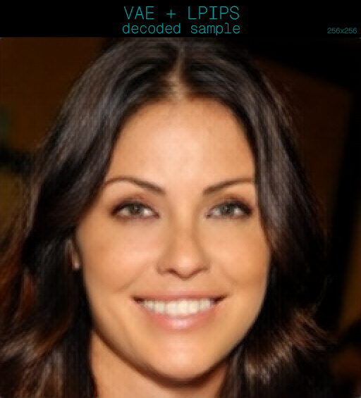
The perceptual loss is a pre-trained model that we use to assess how visually similar the inferred sample is to the original image. It helps to mimic how we may judge the similarity or differences between images as humans. The model is called LPIPS – “Learned Perceptual Image Patch Similarity”.
- LPIPS will be used in a frozen state by loading a previously trained state.
Adversarial Loss
The adversarial loss is a GAN Discriminator that is trained along side the VAE model in the training loop. The discriminator model’s objective is to detect synthetic images.
Dataset
#############################
# Create the dataset
im_dataset_cls = CelebDataset
im_dataset = im_dataset_cls(split ='train',
                            im_path ='data/CelebAMask-HQ',
                            im_size = 256,
                            im_channels = 3)

data_loader = DataLoader(im_dataset,
                         batch_size = 4,
                         shuffle = True)
#############################The class CelebDataset is a custom object that handles importing the training dataset and handles small pre-processing tasks such as converting the images to tensors.
The data set is loaded into a DataLoader to allow the training examples to be distributed in batches of 4 images at a time, allowing for random shuffling to occur on every step of training.
#############################
# Fixed reference images for reconstruction visualization
fixed_idxs = [13]
fixed_im = torch.stack([im_dataset[i] for i in fixed_idxs],
                       dim=0).float().to(device)
#############################- Training Example 13 is hardcoded to ensure we have a single image that we can track visually throughout the training loop.
- This will be used to generate samples every 5 steps.
Loss Functions & Optimizers
#############################
# L2 loss functions
recon_criterion = torch.nn.MSELoss()
disc_criterion = torch.nn.MSELoss()
#############################- Two loss functions are created:
- recon_criterion: Used to calculate the loss in reconstruction for the VAE. This primarily used to train the VAE.
- disc_criterion: Used to calculate the loss for the discriminator. This primarily used to train the discriminator and indirectly incorporated into training the VAE.
#############################
optimizer_g = Adam(model.parameters(),
                   lr=autoencoder_lr,
                   betas=(0.5, 0.999))
optimizer_d = Adam(discriminator.parameters(),
                   lr=autoencoder_lr,
                   betas=(0.5, 0.999))
#############################- Two Adam optimizers are created
- optimizer_g: Optimizes VAE parameters
- Encoder weights
- Decoder weights
- Recieves gradients from:
- Reconstruction loss (MSE)
- KL loss
- Perceptual loss (LPIPS)
- Adversarial loss
- optimizer_d: Optimizes: Discriminator parameters only
- Receives gradients from:
- Real images → target = 1
- Fake (reconstructed) images → target = 0
- Receives gradients from:
Training Loop
#############################
for epoch_idx in range(num_epochs):
    optimizer_g.zero_grad(set_to_none=True)
    optimizer_d.zero_grad(set_to_none=True)

    for im in tqdm(data_loader):
        step_count += 1
        im = im.float().to(device)
        # Forward pass through VAE
output, encoder_output = model(im)- Here we start the two loop statements that will be used to iteratively train the models.
- 1st loop iterates over the number of epochs
- 2nd loop iterates over each image in the training data in batches of 4 images per step.
- optimizers are initializes at zero at the start of each epoch
- Image batches are sent to the device
- The batch is sent to the VAE to execute a forward pass
- one forward pass is comprised of a encode and decode pass.
KL Loss
$$ D_{KL}=-\frac{1}{2}\sum_{i=1}^d(1+log \ \sigma_i^2-\mu_i^2-\sigma_i^2)$$
Where:
- mean -> \(\mu\)
- logvar -> \(log \ \sigma^2\)
- logvar.exp() -> \(\sigma^2\) -> variance
  # encoder_output has 2 * z_channels -> [mu, logvar]
  mean, logvar = torch.chunk(encoder_output, 2, dim=1)

  # KL divergence term: D_KL(q(z|x) || N(0, I))
kl_loss = -0.5 * torch.mean(1 + logvar - mean.pow(2) - logvar.exp())The KL loss measures how different the encoder’s learned latent distribution is from a standard normal distribution.
It compares:
$$q(z|x)=N(\mu(x),\sigma^2(x)) \rightarrow p(z) = N(0,I)$$
The KL terms becomes larger when:
- the mean drifts far from 0
- the variance is very small (over-confident)
- the variance is very large (too spread out)
The term becomes smaller when:
- \(\mu \approx 0\)
- \(\sigma^2 \approx 1\)
- encoder_output: This is the probability distribution produced by the encoder. This is the raw data that gets used to create the latent image.
- encoder_output: Shape (B,C,W,H) , with 8 channels, torch.chunk splits the first 4 channels into mean and the last 4 into log variance.
- kl_loss = -0.5 * torch.mean(1 + logvar – mean.pow(2) – logvar.exp())
- Implementation of the KL loss formular using the \(\mu\) and \(log \ \sigma^2\) components that have been extraced from encoder_output
Sample Export
This block handles sample export during the training process to visually monitor progress over iterations.
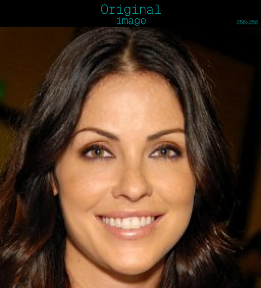
Using a consistent image that we encode and decode into a sample, we export a grid with the original image on the left and the decoded image on the right.
do_export = (step_count % image_save_steps == 0) or (step_count == 1)
if do_export:
    was_training = model.training
    model.eval()
    with torch.no_grad():
        ref_im = fixed_im[0:1]  # (1,3,H,W)
        z_ref, _ = model.encode(ref_im)
        out_ref = model.decode(z_ref)

        inp = ((ref_im + 1) / 2).clamp(0, 1).detach().cpu()        # (1,3,H,W)
        rec = ((out_ref + 1) / 2).clamp(0, 1).detach().cpu()       # (1,3,H,W)

        # [EXP-11] Concatenate horizontally (width axis) -> (1,3,H,2W)
        side_by_side = torch.cat([inp, rec], dim=3)
        img = torchvision.transforms.ToPILImage()(side_by_side.squeeze(0))

        img.save(os.path.join(samples_dir,
                              f'current_autoencoder_sample_{img_save_count}.png'))
        img.close()
        img_save_count += 1
model.train(was_training)- Export occurs on the first step and then every 5th step.
- The following pattern is used to temporarily put the model into eval mode instead of training mode, this ensures deterministic inference behaviour. Some layer can behave differently in training mode vs eval mode, this is good practice.
- was_training = model.training
- model.eval()
- with torch.no_grad(): This saves vram as we do not want to track gradients or build a computation graph during inference.
- We pass our fixed image into a forward pass of the encoder and decoder
ref_im = fixed_im[0:1] # (1,3,H,W)z_ref, _ = model.encode(ref_im)out_ref = model.decode(z_ref)
- The tensor images are converted into displayable image range [0,1], the tensors for training are [-1,0]
inp = ((ref_im + 1) / 2).clamp(0, 1).detach().cpu() # (1,3,H,W)rec = ((out_ref + 1) / 2).clamp(0, 1).detach().cpu() # (1,3,H,W)
- The images are arranged in a side by side grid
- side_by_side = torch.cat([inp, rec], dim=3)
- The tensor has the batch dimension removed (B,C,W,H) -> (C,H,W) via .squeeze(0) and the tensor is converted to a PIL image
- img = torchvision.transforms.ToPILImage()(side_by_side.squeeze(0))
- The remaining lines simply save this image grid to disk and restores the training state of the mode:
model.train(was_training)
Optimize VAE (Generator)
######### Optimize VAE (generator) ##########

# L2 Loss (MSE) Reconstruction loss
recon_loss = recon_criterion(output, im)
recon_loss = recon_loss / autoencoder_acc_steps

# KL loss (already computed above)
g_loss = recon_loss + kl_weight * kl_loss / autoencoder_acc_steps

# Adversarial loss only if disc_step_start steps passed
if step_count > disc_step_start:
    disc_fake_pred = discriminator(output)
    disc_fake_loss = disc_criterion(disc_fake_pred,torch.ones_like(disc_fake_pred))
    g_loss += disc_weight * disc_fake_loss / autoencoder_acc_steps

## Perceptual Loss
lpips_loss = torch.mean(lpips_model(output, im))
g_loss += perceptual_weight*lpips_loss / autoencoder_acc_steps

g_loss.backward()Reconstruction Loss and KL Loss
- recon_criterion(output, im)
- output = reconstructed image from the VAE decoder
im= original input imagerecon_criterion = MSELoss()so this is mean squared error between pixels.
- Divide by gradient accumulation steps, Since .backward() is called multiple times before optimizer_g.step(), the loss is divided by the number of gradient accumulation steps. Because gradients from each .backward() call are summed, this division ensures that the final accumulated gradients match the gradients that would have been produced if the model had been trained with a single large batch and a single .backward() call.
- g_loss = Generator Loss
- kl_loss was computed earlier from the encoder’s mean, logvar.
- You multiply by kl_weight because KL can easily overpower recon loss if not weighted.
- KL_loss is then divide by autoencoder_acc_steps for the same reason as above prior to being added to recon_loss to make g_loss
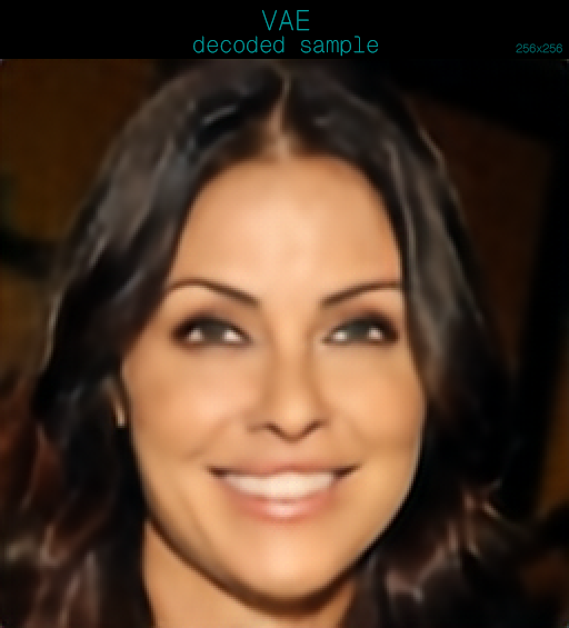
The reconstruction loss measures how similar the decoded image is to the original sample and provides a measure how how accurate the outcome is on a pixel level, while the KL loss encourages the encoder’s latent distribution to stay close to a standard normal making the latent space “well-behaved” and sampleable..
Discriminator Loss
# Adversarial loss only if disc_step_start steps passed
if step_count > disc_step_start:
    disc_fake_pred = discriminator(output)
    disc_fake_loss = disc_criterion(disc_fake_pred,torch.ones_like(disc_fake_pred))
g_loss += disc_weight * disc_fake_loss / autoencoder_acc_steps- The discriminator only kicks in once the training loop has executed more than 15000 steps, This loss term is delayed because early on, reconstructions are trash. If you train the discriminator immediately it can become too good too fast, and the adversarial signal becomes unstable or unhelpful.
- discriminator(output) = produces a “realness score” per image or per batch.
- disc_fake_loss = disc_criterion(disc_fake_pred, torch.ones_like(disc_fake_pred))
- MSE is calculated between the score from the discriminator and a tensor of ones. The closer the discriminator score is to 1 the more convincing the decoded sample is. This is the LSGAN formulation.
- g_loss += disc_weight * disc_fake_loss / autoencoder_acc_steps
- THe disc_fake_loss calculated from the MSE loss function is added to the g_loss by a weight, this controls how much the discriminator competes with the reconstruction loss.
Perceptual Loss
## Perceptual Loss
lpips_loss = torch.mean(lpips_model(output, im))
g_loss += perceptual_weight * lpips_loss / autoencoder_acc_stepsLPIPS compares images in a deep feature space (not raw pixels), approximating human perceptual similarity.
- Pixel MSE punishes small shifts heavily and tends to encourage blurry averages. LPIPS rewards perceptual similarity — “looks the same” rather than “every pixel matches”.
- Again perceptual loss is multiplied by a weight to allow balance over other terms and divided by acc_steps.
g_loss.backward()- g_loss.backward() computes the gradients of the total generator loss with respect to all trainable parameters of the VAE (encoder and decoder), and stores those gradients in the .grad attribute of each parameter.
#############################
if step_count % autoencoder_acc_steps == 0:
    optimizer_g.step()
optimizer_g.zero_grad()Optimize Discriminator
######### Optimize Discriminator #######
if step_count > disc_step_start:
    fake = output
    disc_fake_pred = discriminator(fake.detach())
    disc_real_pred = discriminator(im)
    disc_fake_loss = disc_criterion(disc_fake_pred,torch.zeros_like(disc_fake_pred))
    disc_real_loss = disc_criterion(disc_real_pred,torch.ones_like(disc_real_pred))
    disc_loss = disc_weight * (disc_fake_loss + disc_real_loss) / 2
    disc_loss = disc_loss / autoencoder_acc_steps
    disc_loss.backward()
    ################### Update Discriminator
    if step_count % autoencoder_acc_steps == 0:
        optimizer_d.step()
        optimizer_d.zero_grad(set_to_none=True)
#####################################- The discriminator is activated once the step count is over 15000
    fake = output
    disc_fake_pred = discriminator(fake.detach())
disc_real_pred = discriminator(im)- output: is the reconstructed image sample from the decoder, its copied to a new var and .detached() – this is critical: it stops gradients flowing back into the VAE while you’re training only the discriminator.
- disc_fake_pred & disc_real_pred are the discriminators predictions for both the decoded sample and the original image.
disc_fake_loss = disc_criterion(disc_fake_pred, torch.zeros_like(disc_fake_pred))
disc_real_loss = disc_criterion(disc_real_pred, torch.ones_like(disc_real_pred))- MSE Loss is used as a GAN classification loss:
- fake should map to 0
- real should map to 1
disc_loss = disc_weight * (disc_fake_loss + disc_real_loss) / 2
disc_loss = disc_loss / autoencoder_acc_steps
disc_loss.backward()- Average the two losses and apply a weight to control how much the GAN term matters.
- Since we are accumulating gradients over autoencoder_acc_steps minibatches, we scale loss down so the effective gradient matches “one big batch” training.
- .backward() computes and accumulates gradients into discriminator.parameters().
Update the discriminator
################### Update Discriminator
if step_count % autoencoder_acc_steps == 0:
    optimizer_d.step()
optimizer_d.zero_grad(set_to_none=True)- Every acc_steps minibatches:
- apply the accumulated gradients to update discriminator weights
- clear grads for the next accumulation window
Update the VAE (Generator)
################### Update VAE (Generator)
if step_count % autoencoder_acc_steps == 0:
    optimizer_g.step()
optimizer_g.zero_grad(set_to_none=True)- Every acc_steps minibatches:
- apply the accumulated gradients to update VAE weights
- clear grads for the next accumulation window
Checkpoint block
#############################
# Save model checkpoint after every epoch
torch.save(model.state_dict(), os.path.join(
'celebhq_task_dir',
'vae_ckpt.pth'
))
#############################- The models weights are saved out at the end of each epoch.