
In an effort to understand machine learning from the ground up, the aim of this post is to implement a really simple machine learning system to help understand the fundamentals. “Univariate Linear Regression” is probably the simplest system to implement, it certainly isn’t the most effective for complex problems but it’s a good starting point in understanding machine learning.
Overview
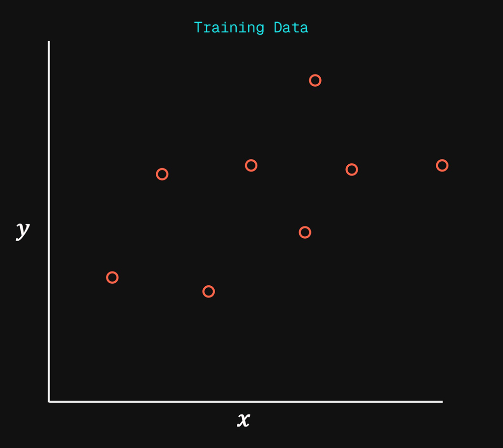
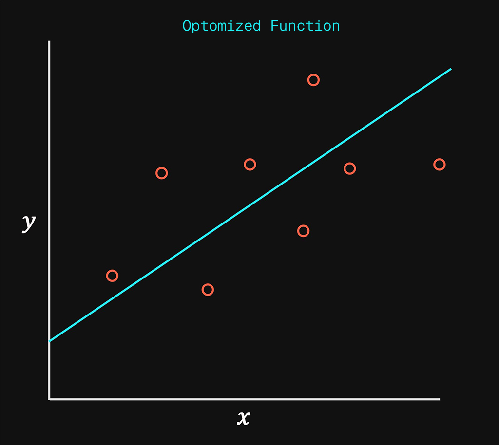
In simple terms all we are trying to achieve, is to take the input data on the left and “fit” a line down the middle of the data points as accurately as possible.
Linear regression is simply creating a straight line to represent existing data points as accurately as possible.
What this enables us to do is provide a method of predicting any value along that straight line as an extrapolation of the input data. The line fills in the missing gaps of data, by approximating that data as a linear distribution.
Use Case:
Let’s say you want to predict a house price based on a single variable. Lets call this variable \(x\) and it will represent the internal square footage of a property. Based on \(x\) the system will attempt to predict the sale price of the house. The output will be referred to as \(y\)
$$ x(ft^2) \rightarrow y(Sale \ Price) $$
The above represents the input or training data on the left and the outcome of the system will be the straight line on the right.
The training data is a sample of the correct relationship between \(x\) and \(y\), it provides the correct value of what \(y\) will be relative to \(x\) for the number of samples in the training data.
Since we are using input data that represents correct output data this system is a supervised learning system.
The input or training data will only have a limited number of correct “answers” of what the sale price (\(y\)) will be when given the size of the property (\(x\)). What our system will provide us is the ability to get a sale price (\(y\)) estimation or prediction of any sized house (\(x\)) even if it falls outside of the data provided by the training data.
if we break down the name “Univariate Linear Regression” it simply means:
- Univariate : Refers to a single variable or feature to be used in training the system, \(x\). If multiple features were to be used it would be multivariate.
- Linear : Refers to the linear function that is used to model the predictions.
- Regression : Is a term from statistics that refers to estimating or predicting the value of one variable based on one or many other variables.
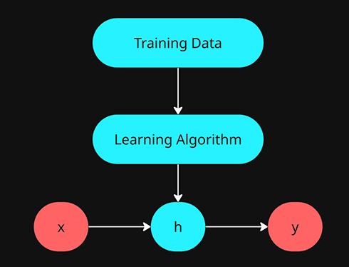
All supervised machine learning systems require the following components:
- Training Data
- Prediction Function
- Hypothesis
- Error Evaluation
- Cost or Loss Function
- Learning Algorithm
- Gradient Descent
Data Representation
- \(m\) = Number of training data samples
- \(x\) = Input variable or input feature
- \(y\) = Output variable or target variable
- \((x^{(i)},y^{(i)});i=1,…,m\) = This represents the entire set of training data from 1 to 5.
- \(x=y=\mathbb{R}\)
Hypothesis
The hypothesis represents how we will be predicting the output values \(\hat{y}\) given \(x\).
- Hypothesis = \(h\)
- \(h\) effectively produces \(\hat{y}\) given \(x\).
- H is a function that converts any \(x\) input into the predicted value \(\hat{y}\)
- \(\hat{y}\) will represent the predicted data and \(y\) will represent the real data found in the training examples.
H representation
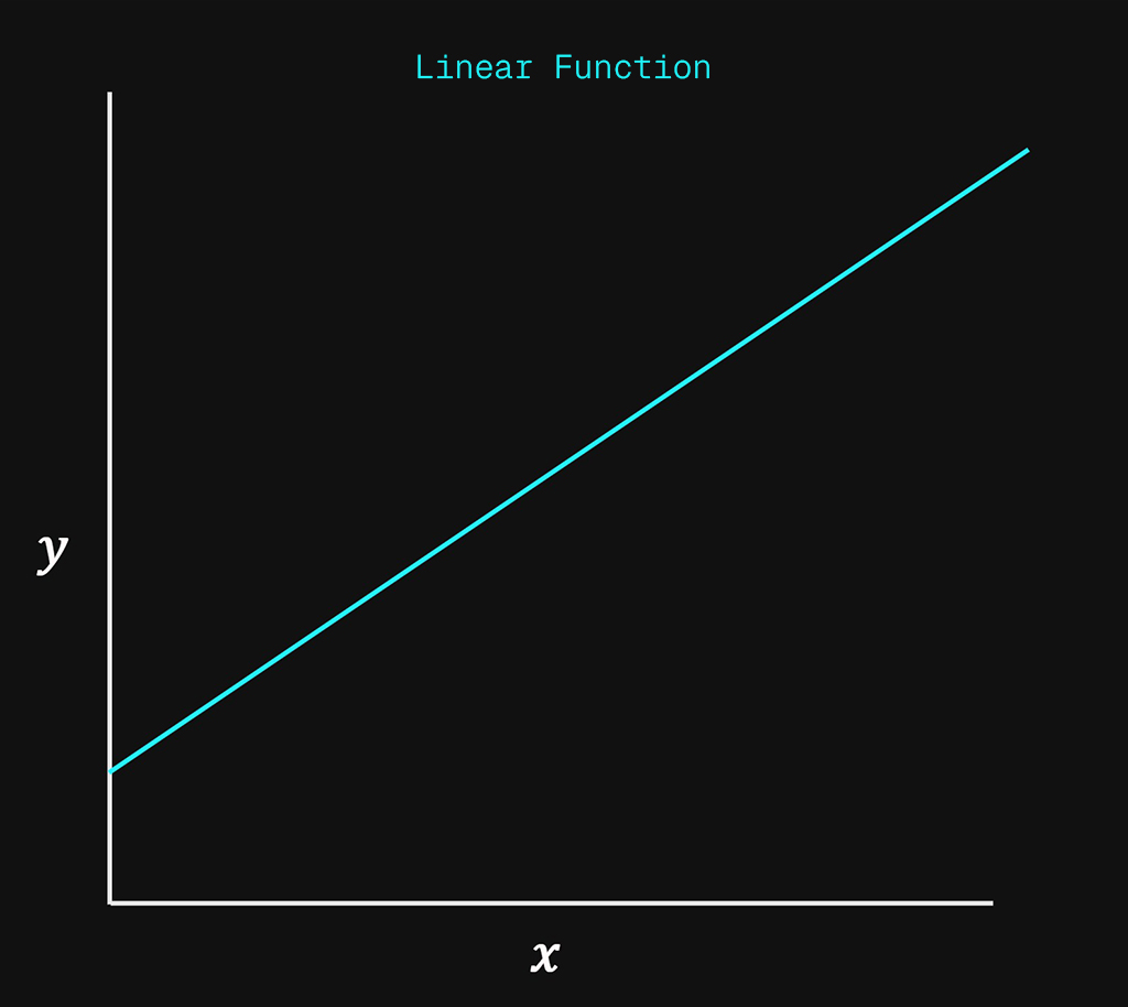
H will be represented by a linear function. Which produces a straight line when charted with respect to \(x\).
$$h_{\theta}(x) = \theta_0 + \theta_1x$$
This is the standard linear function \(f(x)=mx+b\)
- This function produces a linear line that will be adjusted to best fit the training data.
- The function takes \(x\) as input and produces the \(\hat{y}\) output value.
- Shorthand: \(h(x)\)
- \(\theta_0 \ \& \ \theta_1\): These are the two parameters the system will try to optimize to increase the alignment of the linear function to the data set. Which will in turn produce more accurate predictions.
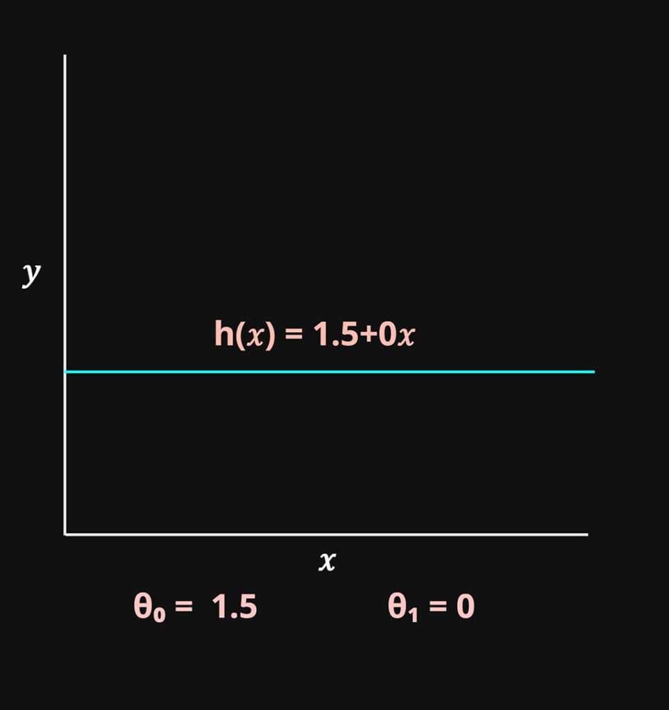
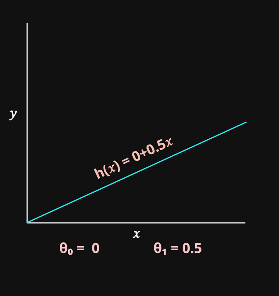
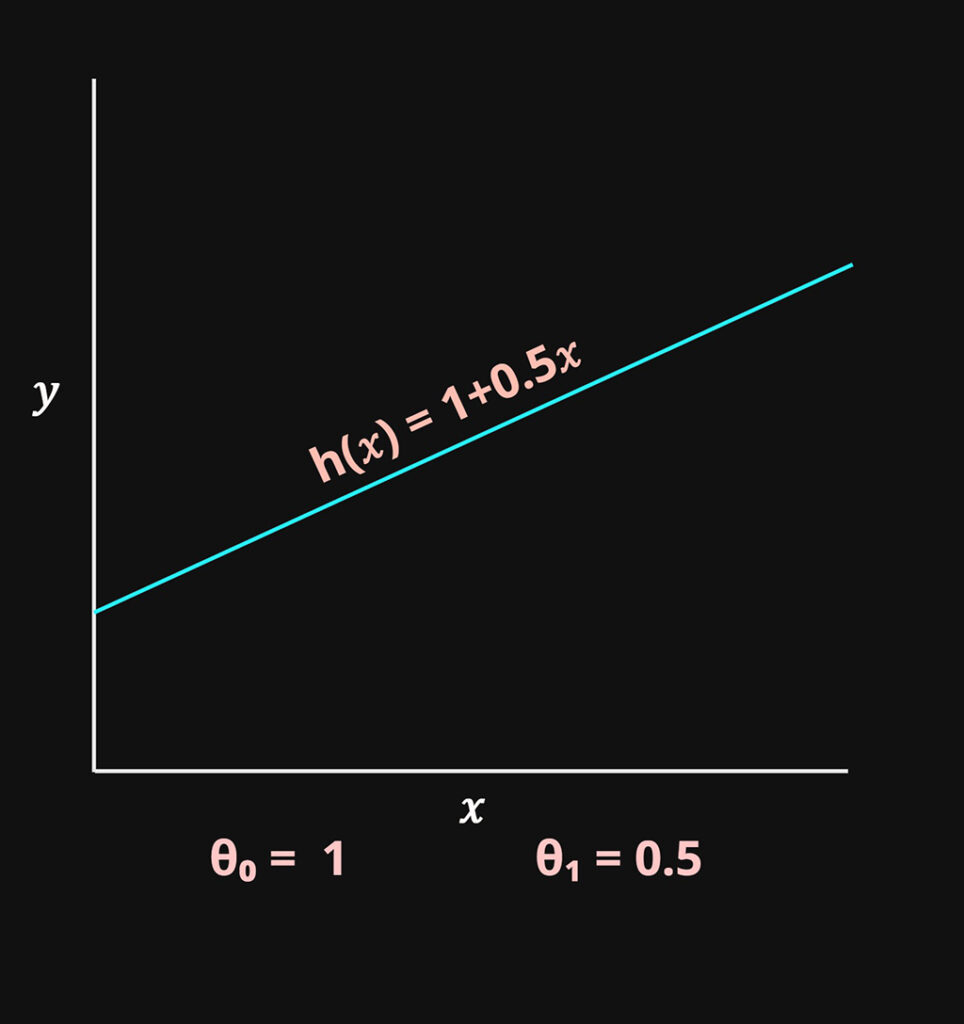
\(\theta_0\) = Controls the y intercept of the function
\(\theta_1\) = Controls the slope of the function
These two variables will be the parameters that will be optimized in the model.
Cost Function
The cost function measures the amount of error or loss between the prediction function and the real data. Its a measure of the difference between the prediction produced by \(h\) to the \(y\) values in the training data.
This may be referred to as the cost , loss or error.
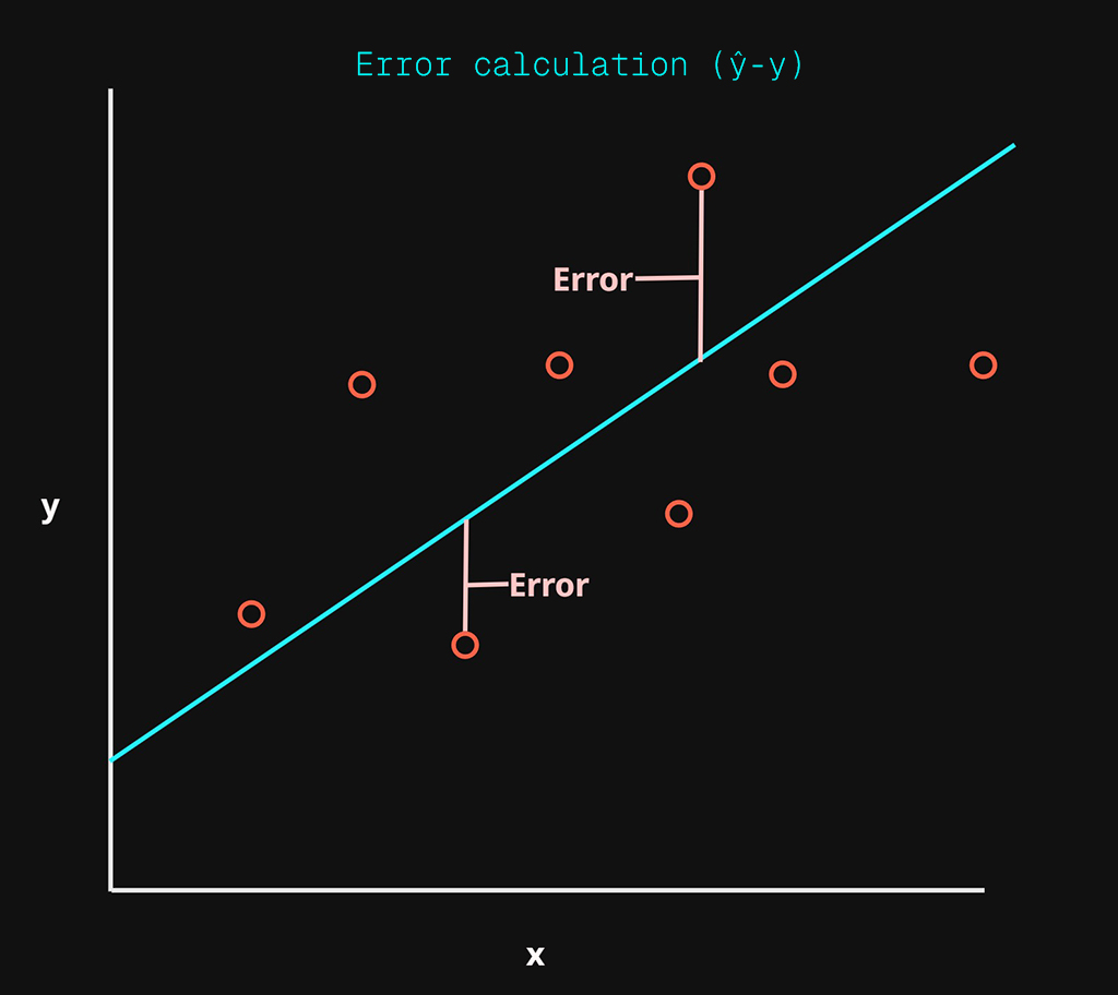
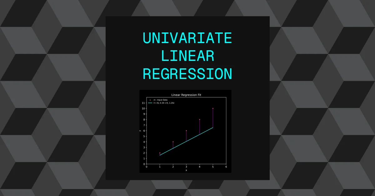
In the above chart, there are three main things to note:
- Training Data: red dots
- Linear function (\(h\)): cyan line
- Error: purple lines
The cyan line is our hypothesis \(h\) which is the linear function and the error is the difference between the predicted \(\hat{y}\) produced by the linear function and the real \(y\) data found in the training examples.
The smaller the cost function or error, the more accurate the system will be at predicting the output value \(\hat{y}\). This cost function is how we measure the performance of the learning algorithm.
We’ll be using Mean Squared Error (MSE) as our cost function.
$$\frac{1}{m}\sum_{i=1}^m(\hat{y}^{(i)}-y^{(i)})^2$$
lets break this down:
- \(\hat{y}^{(i)}-y^{(i)}\) : This delta is the error itself, for every training example \(i\), We are calculating the difference between the predicted output \(\hat{y}\) and the real output value \(y\).
- \(\hat{y}^{(i)}\): This is the output from our hypothesis / linear function \(h_{\theta}(x^{(i)})\). Calculated over each \(x\) found in the training examples.
- The error calculated from the above is squared which either reduces a smaller error or exaggerates larger errors. It also removes any negative errors from the calculation.
- This squared error summed \(\sum_{i=1}^m\) together before being averaged via the multiplication of \(\frac{1}{m}\), remember \(m\) represents the total number of examples in the training data.
- This is know as the Mean Squared Error (MSE)
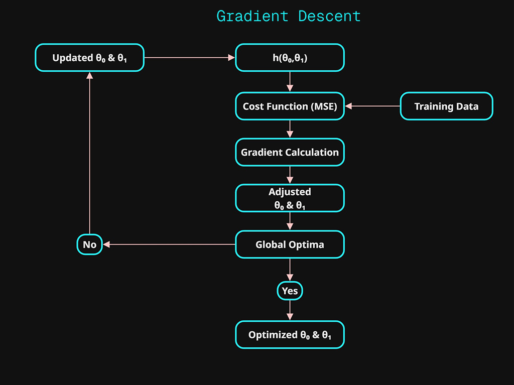
Gradient Descent
Now that we have a function that can be used to represent our predictions \(h\) and we have a method of evaluating the error (MSE). We can focus on the algorithm that will recursively optimize our function to reduce the error. This is how the system will “learn”. The aim is to minimize the cost function.
Machine Learning is about optimizing parameter(s) to reduce the error.
In our linear function \(h\) , we have two parameters that can be adjusted that changes output of \(\hat{y}\). The two parameters are \(\theta_0 \ \& \ \theta_1\).
To simplify our understanding, lets focus on a single parameter \(\theta_0\).
If we chart the result of the cost function (MSE) relative to \(\theta_0\). We can see what the outcome of the cost function would be for the range of possible values for \(\theta_0\)
This would create the parabola shown as the error (cost function) below. This is the gradient descending.
Gradient Descent Process:
- Calculate the cost function at the initial value for \(\theta_0\).
- Finds the gradient. This is the slope calculated from the derivative.
The slope will represent the rate of change at that current \(\theta_0\) position. This will give both a direction and magnitude that will be used to adjust \(\theta_0\). - The gradient is multiplied by a learning rate \(\alpha\) and then used to update \(theta_0\). This becomes the adjusted parameter that is used in the next iteration (epoch).
The smallest cost function possible is referred to as the global optima. The global optima is the most optimized value for \(\theta_0\) as it will produce the lowest error.
This how the “learning” works. Every step of the algorithm will calculate the gradient using derivatives, which is in turn used to adjust the parameter(s) in order to reduce the cost function. As the system approaches the global optima, the rate of change calculated by the derivative will automatically reduce in magnitude which in turn will decreases the amount of adjustment that takes place to \(\theta_0\).
Learning Rate & Iterations
Using a learning algorithm such as gradient descent, there are two main ways to control how efficient the system is.
- \(\alpha\): Learning Rate
- Epoch: Learning Iterations
The learning rate is a coefficient used to multiply the gradient prior to it adjusting the parameter(s). If the learning rate is too low you will require excessive epochs to achieve the global optima.
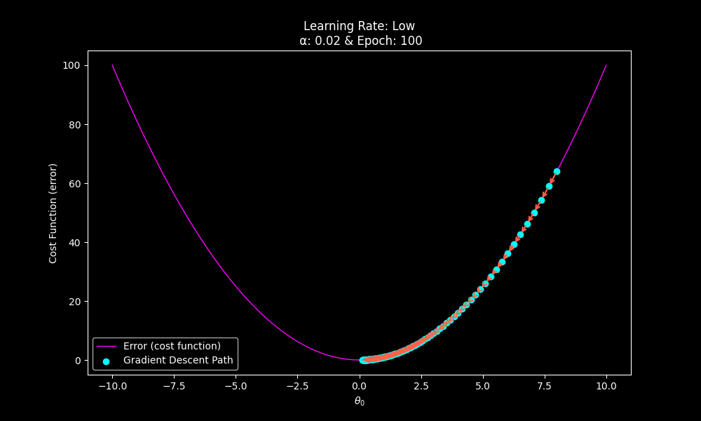
The local optima requires more iterations as a result of the low learning rate.
If the learning rate is too high, even with a large number of epochs, the gradient descent algorithm will never achieve the global optima, as the gradient is being multiplied too high and the parameters will constantly overshoot the most optimum value.
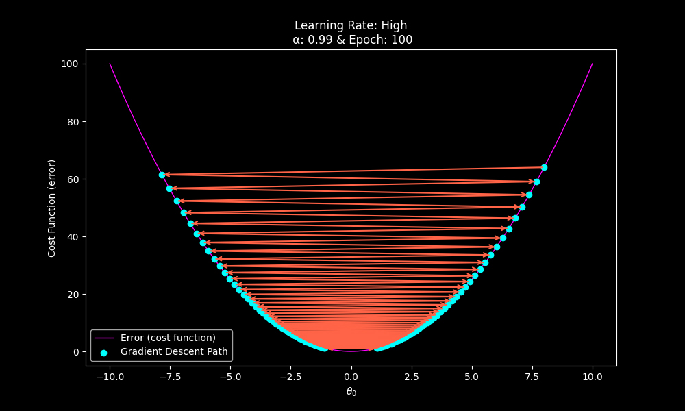
Local optima will never be achieved due to overshooting.
Adjusting the learning rate and epoch will result in optimizing the system efficiently.
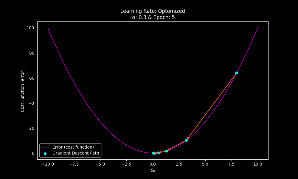
With a more suitable learning rate, far fewer iterations may be required.
Implementation
Lets implement each stage to see how it comes to together.
- Training Data
- Prediction Function
- Hypothesis
- Error Evaluation
- Cost or Loss Function
- Learning Algorithm
- Gradient Descent
1.Training Data
In order to test the algorithm, we will use this super simple set training data.
The data is derived from the linear function: \(f(x) = mx + b\). Real data will likely not be perfectly represented as a linear function.
- \(x=1,2,3,4,5\)
- \(m\) = 2 (slope)
- \(b\) = 0 (y-intercept)
- \(y=2\cdot x + 0\)
| \(x \ (ft^2)\) | \(y \ (Sale \ Price)\) |
| 1 | 2 |
| 2 | 4 |
| 3 | 6 |
| 4 | 8 |
| 5 | 10 |
Because we are synthetically creating this simple data set, we know exactly what the results of the linear regression model need to be in order for it to be perfectly accurate. The closer we get to the above linear function the better.
# Training Data
def generate_training_data():
    # y = 2x+0
    # slope = 2
    # y-intercept = 0
    x = np.array([1, 2, 3, 4, 5], dtype=float)
    y = np.array([2, 4, 6, 8, 10], dtype=float)  # y = 2x
    return x,y
2.Prediction Function
H will be represented by a linear function. Which produces a straight line when charted with respect to \(x\).
$$h_{\theta}(x) = \theta_0 + \theta_1x$$
# Prediction function
def predict(x, theta_0, theta_1):
    # linear function
    # theta_0 = y-intercept
    # theta_1 = slope
    return theta_0 + theta_1 * x
3.Error Evaluation
We’ll be using Mean Squared Error (MSE) as our cost function.
$$\frac{1}{m}\sum_{i=1}^m(\hat{y}^{(i)}-y^{(i)})^2$$
# Error function
def compute_mse(y_true, y_pred):
    # MSE cost function
    return ((y_true - y_pred) ** 2).mean()
4.Learning Algorithm
Gradient Descent Function
# Learning algorithm
def gradient_descent(x, y, learning_rate, epochs):
    # Gradient descent function

    # Initial paramter values
    theta_0 = 0.0
    theta_1 = 0.0

    # number of trainding data samples
    m = len(y)

    # Iteration cycle per epoch
    for epoch in range(epochs):

        # y prediction based on current parameter values used
        # in linear function
        y_pred = predict(x, theta_0, theta_1)
        # error (delta) between current linear function and
        # sample data.
        error = y_pred - y

        # Gradients: magnitude relative to size of error
        d_theta_0 = (2/m) * np.sum(error)
        d_theta_1 = (2/m) * np.sum(error * x)

        # Update parameters using the learning rate as
        # coefficient
        theta_0 -= learning_rate * d_theta_0
        theta_1 -= learning_rate * d_theta_1

    # Calculate MSE for evaualtion
    mse = compute_mse(y, y_pred)
    # Return the optomized parameters and MSE
    return theta_0, theta_1, mse
Running the model
To run the algorithm we will first use the following inputs.
Inputs:
- Training Data: in this case our simple linear distribution of points based on a linear function with a slope of 2 and y-intercept of 0.
- Learning rate = 0.001
- Epochs = 248
##### Synthetic training data
x , y = generate_training_data()

##### Run Gradient Descent
learning_rate=0.001
epochs=248
theta_0, theta_1, mse = gradient_descent(x, y, learning_rate , epochs)

###### Present results
## Using an epsilon of 1e-6
theta_0_r = np.round(theta_0, 6)
theta_1_r = np.round(theta_1, 6)
mse_r = np.round(mse, 6)

##### Output results
print(f'theta_0 = {theta_0_r}\ntheta_1 = {theta_1_r}\nmse = {mse_r}\n')
This gives us the following output:
theta_0 = 0.471753
theta_1 = 1.864061
mse = 0.041089
Using this particular combination of learning rate and number of iterations (epochs) we get a high level of error.
The parameters have had mixed results in terms of optimisation.
- theta_0: Worst than starting value of zero
- theta_1: Fairly decent, considering our target is 2
- mse: Reflects a high level of error.
Remember that since we are using training data that has been derived from the linear function: \(y=2\cdot x + 0\)
We know that in order for this model to be perfectly fit, theta_0 which represents the y-intercept of the prediction function must be 0 and theta_1 which represent the slope must be 2.
Here is a visual representation of the learning algorithm adjusting the prediction function and the error rate decreasing as the learning algorithm improves.
A perfectly matched prediction function would look like this.
theta_0 = 0.0
theta_1 = 2.0
mse = 0.0
Visually we can see that the prediction function aligns with the test data perfectly now.
Since the prediction function and the test data we are using are both essentially the same linear function. We know that this algorithm works, as this control test allows use to ensure it does mathematically. Both functions are identical at this point.
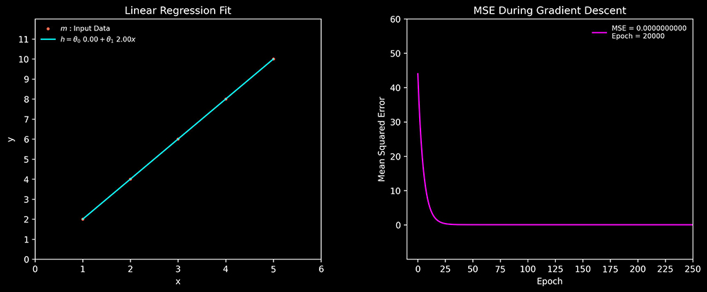
This was achieved by using the following values.
- Learning rate = 0.004
- Epochs = 20000
Complete python code
"""
Univariate Linear Regression Model
"""
import numpy as np

# Learning algorithm
def gradient_descent(x, y, learning_rate, epochs):
    # Gradient descent function

    # Initial paramter values
    theta_0 = 0.0
    theta_1 = 0.0

    # number of trainding data samples
    m = len(y)

    # Iteration cycle per epoch
    for epoch in range(epochs):

        # y prediction based on current parameter values used in linear function
        y_pred = predict(x, theta_0, theta_1)
        # error (delta) between current linear function and sample data.
        error = y_pred - y

        # Gradients: magnitude relative to size of error
        d_theta_0 = (2/m) * np.sum(error)
        d_theta_1 = (2/m) * np.sum(error * x)

        # Update parameters using the learning rate as coefficient
        theta_0 -= learning_rate * d_theta_0
        theta_1 -= learning_rate * d_theta_1

    # Calculate MSE for evaualtion
    mse = compute_mse(y, y_pred)
    # Return the optomized parameters and MSE
    return theta_0, theta_1, mse

# Prediction function
def predict(x, theta_0, theta_1):
    # linear function
    # theta_0 = y-intercept
    # theta_1 = slope
    return theta_0 + theta_1 * x

# Error function
def compute_mse(y_true, y_pred):
    # MSE cost function
    return ((y_true - y_pred) ** 2).mean()

# Training Data
def generate_training_data():
    # y = 2x+0
    # slope = 2
    # y-intercept = 0
    x = np.array([1, 2, 3, 4, 5], dtype=float)
    y = np.array([2, 4, 6, 8, 10], dtype=float)  # y = 2x
    return x,y

def main():

    ##### Synthetic training data
    x , y = generate_training_data()

    ##### Run Gradient Descent
    learning_rate=0.001
    epochs=248
    theta_0, theta_1, mse = gradient_descent(x, y, learning_rate , epochs)

    ###### Present results
    ## Usineg an epsilon of 1e-6
    theta_0_r = np.round(theta_0, 6)
    theta_1_r = np.round(theta_1, 6)
    mse_r = np.round(mse, 6)

    ##### Output results
    print(f'theta_0 = {theta_0_r}\ntheta_1 = {theta_1_r}\nmse = {mse_r}\n')


if __name__ == "__main__":
    ###### Run
    main()