

Note: This study is still in progress. Consider it a rough draft.
Latent Diffusion Models were first introduced in the 2022, in the academic paper: “High-Resolution Image Synthesis with Latent Diffusion Models” https://arxiv.org/pdf/2112.10752
The paper introduces the idea of converting images into latent space prior to training/inference stage. This greatly improved performance and allowed the way for much larger resolution images being able to be synthesized with a diffusion model.
A LDM can be thought of as a DDPM with the following additional elements:
LDM = DDPM + Autoencoder + CLIP + Cross-Attention
Some of the these components have been previously broken down into detail, this study will be focusing on bringing all the elements together along with exploring anything that has not previously been studied.
Lets touch on what has been previously covered.
DDPM (Denoising Diffusion Probabilistic Model)
- The DDPM is what carries out the generation of novel images based on statistical distribution learned from training data.
- This is the main framework that controls what is being created through inference and if any conditioning is used for control.
I’ve carried out a separate study of this model here:
This DDPM study covers mainly the high level concepts and training of a DDPM (unconditional). However the UNet itself is not covered in any depth. Its worth noting that this original implementation of a DDPM is in pixel space, however the architecture is largely the same otherwise.
Autoencoder = Encodes or Decodes to and from Latent Space
Cross Attention = Introduces conditioning such as text and/or otherwise.
VAE (Variational Autoencoder)
- The VAE takes care of two important operations: Encoding and Decoding Images to and from pixel space <-> latent space.
- Latent Image greatly improves the performance, making larger spatial resolutions possible.
Again, I’ve carried out two separate deep dives on VAEs that does into detail on both the training and also actual neural network model that is used to make converting between pixel space to latent space and visa versa.
In this study what we will be diving into is how these all come together along with how the actual UNet works along with introducing conditioning to demonstrate how control can be introduced.
This study will be using python implementations that was created by Tushar Kumar. The original code can be found in the GitHub link below:
https://github.com/explainingai-code/StableDiffusion-PyTorch
CLIP (Contrastive Language–Image Pretraining)
CLIP is a pretrained model that bridges the gap between images and language. It is used to give visual concepts linguistic meaning and connect language to visual concepts.
Its a pre-trained model that comprises of two types of encoders one for images -> image embeddings and text -> text embeddings. LDM utilizes the text encoder to create text embeddings that are used for text conditioning within the diffusion process. I’ve previously covered this topic as a basic introduction below.
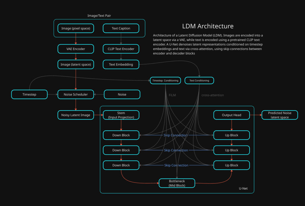
The LDM
The model we will be going over is a LDM with text conditioning. It utilizes the same logic of a DDPM with two exceptions. The UNet operates in latent space not pixel space and we are going to be using text conditioning which is done through cross-attention within the UNet.
As previously mentioned VAEs and DDPMs have been covered in detail previously so this study will be focusing on the differences that previously delved into.
Unlike a conventional DDPM implementation, the LDM has multiple models that need prior training. The important distinction in workflow with a LDM is the image dataset that will be used for training is not directly used for training the UNet model used by DDPM. The image training set is what the VAE model will be trained on directly and the latents the VAE encoding produces is what the DDPM UNet will be trained on with diffusion.
Lets jump into training the LDM.
Training
def train():

    ########## Create the noise scheduler #############
    scheduler = LinearNoiseScheduler(num_timesteps = 1000,
                                     beta_start = 0.00085,
                                     beta_end = 0.012)
    ###############################################

    # Instantiate Condition related components
    text_tokenizer = None
    text_model = None
    empty_text_embed = None

    with torch.no_grad():
        text_tokenizer = CLIPTokenizer.from_pretrained('openai/clip-vit-base-patch16')
        text_model = CLIPTextModel.from_pretrained('openai/clip-vit-base-patch16').to(device)
empty_text_embed = get_text_representation([''], text_tokenizer, text_model, device)- LinearNoiseScheduler: This is the standard noise scheduler that we have covered in the DDPM study.
- CLIPTokenizer: This will be used to convert strings -> token IDs
- CLIPTextModel: CLIP text transformer this converts tokens -> Embeddings
- get_text_representation(): embedding for an empty prompt [”]
- This is for classifier-free guidance (CFG) training. Text labels will be occasionally dropped and replaced with empty prompt embedding so the models learns both conditional and unconditional denoising.
    condition_config = {'condition_types': ['text']}

    im_dataset_cls = CelebDataset

    im_dataset = im_dataset_cls(split='train',
                                im_path='data/CelebAMask-HQ',
                                im_size=256,
                                im_channels=3,
                                use_latents=True,
                                latent_path=os.path.join('celebhq',
                                                         'vqvae_latents'),
                                condition_config=condition_config)

    data_loader = DataLoader(im_dataset,
                             batch_size=16,
shuffle=True)- The standard dataset and DataLoader prep work, the only exception is the dataset has a matching text label for each image in the training dataset.
    # Instantiate the unet model
    model = Unet().to(device)
    model.train()
    # Instantiate the VAE model
    vae = VAE().to(device)
    vae.eval()

    # Load the pre-trained weights for the VAE
    vae.load_state_dict(torch.load(os.path.join('celebhq', 'vae_ckpt.pth'),map_location=device))

    for param in vae.parameters():
param.requires_grad = False- Initiate both the UNet and VAE. The VAE has been previously trained on the training data set.
    # Specify training parameters
    num_epochs = 100
    optimizer = Adam(model.parameters(), lr=0.000005)
    criterion = torch.nn.MSELoss()

    # Run training
    for epoch_idx in range(num_epochs):
        losses = []
        for data in tqdm(data_loader):
            im, cond_input = data
            optimizer.zero_grad()
            im = im.float().to(device)
            with torch.no_grad():
im, _ = vae.encode(im)- The loss criteria and optimizer are initialized
- The main training loop is established, here you see the standard format with both the epoch outer loop and the training batch inner loop.
- The main difference between this and the standard DDPM approach is the the use of the VAE to encode the training examples batch from pixel space into latent space.
- Each batch has two types of data:
- im = this is the batch of images in pixel space
- cond_input = these are text labels that will be used as prompts for each image. Each image in the batch has its own label that will be used in training.
          ########### Handling Conditional Input ###########

          with torch.no_grad():
              assert 'text' in cond_input, 'Conditioning Type Text but no text conditioning input present'

              text_condition = get_text_representation(cond_input['text'],
                                                              text_tokenizer,
                                                              text_model,
                                                              device)
              text_drop_prob = 0.1
              text_condition = drop_text_condition(text_condition, im, empty_text_embed, text_drop_prob)
              cond_input['text'] = text_condition

################################################- get_text_representation(): This is what will take the labels for each image and convert them into CLIP text embeddings
Lets jump into this function to see what is going on
def get_text_representation(text,
                            text_tokenizer,
                            text_model,
                            device,
                            truncation=True,
                            padding='max_length',
                            max_length=77):


    # Convert text to tokens
    token_output = text_tokenizer(text,
                                  truncation=truncation,
                                  padding=padding,
                                  return_attention_mask=True,
                                  max_length=max_length)

    # Extract the token ids and teh attention mask
    indexed_tokens = token_output['input_ids']
    att_masks = token_output['attention_mask']

    # Convert both to tensors on the device
    tokens_tensor = torch.tensor(indexed_tokens).to(device)
    mask_tensor = torch.tensor(att_masks).to(device)

    text_embed = text_model(tokens_tensor, attention_mask=mask_tensor).last_hidden_state

    return text_embed
text: list of strings, length = batch size- Example:
["a smiling face", "a person wearing glasses"] text_tokenizer: CLIP tokenizer (string → token IDs)text_model: CLIP text encoder (tokens → embeddings)device: CPU or GPUmax_length=77: CLIP’s fixed context length
Tokenization
- truncation=True → If text is longer than 77 tokens, extra tokens are discarded.
- padding=’max_length’ → Shorter prompts are padded with special padding tokens.
- return_attention_mask=True → Creates a mask so CLIP knows which tokens are real vs padding.
token_output = {
    'input_ids':       [B, 77],
    'attention_mask':  [B, 77]
}- input_ids: the converted token ids
- attention_mask: a binary mask per token to determine what is a real token and what is a padding:
- 1 -> real token
- 0 -> padding token
text_embed = text_model(tokens_tensor, attention_mask=mask_tensor).last_hidden_state- This runs the CLIP text encoder:
- Looks up token embeddings
- Adds positional embeddings
- Passes them through a Transformer encoder
- Outputs contextualized embeddings for every token
- .last_hidden_state: This returns embeddings for each token, not a pooled vector.
- text_embed: [B, 77, 512]
- 77 = number of tokens
- 512 = CLIP text embedding dimension
            # Sample random noise
            noise = torch.randn_like(im).to(device)

            # Sample timestep
            t = torch.randint(0, 1000, (im.shape[0],)).to(device)

            # Add noise to images according to timestep
            noisy_im = scheduler.add_noise(im, noise, t)
            noise_pred = model(noisy_im, t, cond_input=cond_input)
            loss = criterion(noise_pred, noise)
            losses.append(loss.item())
            loss.backward()
            optimizer.step()

        print('Finished epoch:{} | Loss : {:.4f}'.format(
                                                        epoch_idx + 1,
                                                        np.mean(losses)))
        torch.save(model.state_dict(), os.path.join('celebhq',
                                                    'ddpm_ckpt_text_cond_clip.pth'))

print('Done Training ...')The remaining block of code for the training loop should look very familiar to what has been covered in the DDPM study, The two main differences are:
- The noise is added to the latent image not the pixel space image, the noisy latent is then passed directly to the UNet
- The UNet also receives the CLIP text embeddings to be used for cross-attention within the model.
The UNet
A diffusion U-Net is a CNN-based encoder–decoder with skip connections, augmented with:
- time conditioning (timestep embeddings)
- attention blocks (self-attention)
- cross-attention (for text or other conditioning)
The classic U-Net structure is the following:
- Down path: reduce spatial size, increase channels → global structure
- Up path: increase spatial size, refine details
- Skip connections: re-inject high-frequency detail from earlier layers
Down Path (encoder)
- Input Latent: 32×32×4
- conv_in: 32×32×4
- Out -> 32×32×256
- U-Net Skip 0
- 32×32×256 -> Stored
- Down Block 0: 32×32×256
- ResBlock
- ResBlock
- Self-Attention
- Cross-Attention
- Downsample
- Out -> 16×16×384
- U-Net Skip 1
- 16×16×384 -> Stored
- Down Block 1: 16×16×384
- ResBlock
- ResBlock
- Self-Attention
- Cross-Attention
- Downsample
- Out -> 8×8×512
- U-Net Skip 2
- 8×8×512 -> Stored
- Down Block 2: 8×8×512
- ResBlock
- ResBlock
- Self-Attention
- Cross-Attention
- Downsample
- Out -> 4×4×768
Bottleneck
- Mid Block 4×4×768
- ResBlock
- ResBlock
- Self-Attention
- Cross-Attention
- Out -> 4×4×512
Up Path (decoder)
- Up Block 0 4×4×768
- Upsample
- -> 8×8×512
- Concat U-Net Skip 2
- 8×8×(512+512) -> 8×8×1024
- ResBlock
- ResBlock
- Self-Attention
- Cross-Attention
- Out -> 8×8×384
- Upsample
- Up Block 1 8×8×384
- ◦ Upsample
- -> 16×16×384
- Concat U-Net Skip 1
- 16×16×(384+384) -> 16×16×768
- ResBlock
- ResBlock
- Self-Attention
- Cross-Attention
- Out -> 16×16×256
- ◦ Upsample
- Up Block 2 16×16×256
- Upsample
- -> 32×32×256
- Concat U-Net Skip 0
- 32×32×(256+256) -> 32×32×512
- ResBlock
- ResBlock
- Self-Attention
- Cross-Attention
- Out -> 32×32×128
- Upsample
Output Head
- GroupNorm
- SiLU
- conv_out: 32×32×128
- Out -> 32x32x4
- Predicted Noise in Latent Space
- Out -> 32x32x4
Lets jump into the code
import torch
import torch.nn as nn
from models.blocks import get_time_embedding
from models.blocks import DownBlock, MidBlock, UpBlockUnet

class Unet(nn.Module):
    def __init__(self):
        super().__init__()

        # Initial convolution layer -> Increase depth (channels)
        self.conv_in = nn.Conv2d(in_channels = 4, out_channels = 256, kernel_size = 3, padding = 1)

        # Initial projection from sinusoidal time embedding
        self.t_proj = nn.Sequential(
            nn.Linear(512, 512),
            nn.SiLU(),
            nn.Linear(512, 512)
)- The U-Net model initializes in the standard torch format.
- conv_in: Expands the channel dimensionality of the latent ahead of feature map extraction and spatial resolution reduction.
- t_proj: turns a fixed sinusoidal timestep embedding into a learned, task-specific time-conditioning vector that modulates the U-Net’s behavior at every layer.
Down Blocks
- Spatial Resolution Reduction
- Channel depth expansion
- Time embedding conditioning
- Self-attention
- cross-attention
        # Build the Downblocks
        self.down_block_0 = DownBlock(
            in_channels = 256,
            out_channels = 384,
            t_emb_dim = 512,
            down_sample = True,
            num_heads = 16,
            num_layers = 2,
            attn = True,
            norm_channels = 32,
            cross_attn = True,
            context_dim = 512
            )

        self.down_block_1 = DownBlock(
            in_channels = 384,
            out_channels = 512,
            t_emb_dim = 512,
            down_sample = True,
            num_heads = 16,
            num_layers = 2,
            attn = True,
            norm_channels = 32,
            cross_attn = True,
            context_dim = 512
            )

        self.down_block_2 = DownBlock(
            in_channels = 512,
            out_channels = 768,
            t_emb_dim = 512,
            down_sample = True,
            num_heads = 16,
            num_layers = 2,
            attn = True,
            norm_channels = 32,
            cross_attn = True,
            context_dim = 512
)- These down blocks are very similar to the down blocks used in the VAE study. We will look at the differences that have been added for the U-Net and text conditioning.
- in_channels , out_channels , num_layers, norm_channels and down_sample is the same as what has been seen in the VAE.
- t_emb_dim: This determines the channels dimensionality of the time embedding.
- attn: This enables self-attention, enabling a global receptive field to improve larger scale context.
- cross_attn: This enables cross-attention, allowing for text conditioning
- context_dim: This configures the cross-attention module with the text embedding’s dimensional depth.
Mid Block
- Channel depth reduction
- Time embedding conditioning
- Self-attention
- cross-attention
        # Build the MidBlock
        self.mid_block_0 = MidBlock(
            in_channels = 768,
            out_channels = 512,
            t_emb_dim = 512,
            num_heads=16,
            num_layers=2,
            norm_channels=32,
            cross_attn = True,
            context_dim = 512
)- Similar to the Down Block in terms of configuration. However self-attention is enabled by default so there is no argument to switch this on/off. The spatial resolution is not modified in this block.
Up Block
- Spatial Resolution Expansion
- Channel depth reduction
- Time embedding conditioning
- Self-attention
- cross-attention
- U-Net skip connections concatenation
        # Build the UpBlocks
        self.up_block_0 = UpBlockUnet(
            in_channels = 512 * 2,
            out_channels = 384,
            t_emb_dim = 512,
            up_sample=True,
            num_heads=16,
            num_layers=2,
            norm_channels=32,
            cross_attn=True,
            context_dim= 512
            )

        self.up_block_1 = UpBlockUnet(
            in_channels = 384 * 2,
            out_channels = 256,
            t_emb_dim = 512,
            up_sample=True,
            num_heads=16,
            num_layers=2,
            norm_channels=32,
            cross_attn=True,
            context_dim= 512
            )

        self.up_block_2 = UpBlockUnet(
            in_channels = 256 * 2,
            out_channels = 128,
            t_emb_dim = 512,
            up_sample=True,
            num_heads=16,
            num_layers=2,
            norm_channels=32,
            cross_attn=True,
            context_dim= 512
)- very similar to the downblocks , with the exception that the up sample happens at the beginning of the block, enabling the larger spatial resolution ahead of the resnet blocks and attention blocks.
- in_channels: This is multiplied by 2, has the latent data that has been stored during the down path is concatenated back into the main latent data path in order to restored high frequency detail.
Output Head
        self.norm_out = nn.GroupNorm(32, 128)
        self.conv_out = nn.Conv2d(in_channels = 128, out_channels = 4, kernel_size=3, padding=1)
    def forward(self, x, t, cond_input=None):
        # B x C x H x W
        out = self.conv_in(x)

        # t_emb -> B x t_emb_dim
        t_emb = get_time_embedding(torch.as_tensor(t).long(), 512)
        t_emb = self.t_proj(t_emb)


        context_hidden_states = cond_input['text']

        # down_outs  [B x C1 x H x W, B x C2 x H/2 x W/2, B x C3 x H/4 x W/4]
        # out B x C4 x H/4 x W/4

        down_outs_0 = out
        out = self.down_block_0(out, t_emb, context_hidden_states)

        down_outs_1 = out
        out = self.down_block_1(out, t_emb, context_hidden_states)

        down_outs_2 = out
        out = self.down_block_2(out, t_emb, context_hidden_states)

        # out B x C3 x H/4 x W/4
        out = self.mid_block_0(out, t_emb, context_hidden_states)

        # out [B x C2 x H/4 x W/4, B x C1 x H/2 x W/2, B x 16 x H x W]
        out = self.up_block_0(out, down_outs_2, t_emb, context_hidden_states)
        out = self.up_block_1(out, down_outs_1, t_emb, context_hidden_states)
        out = self.up_block_2(out, down_outs_0, t_emb, context_hidden_states)

        out = self.norm_out(out)
        out = nn.SiLU()(out)
        out = self.conv_out(out)
        # out B x C x H x W
        return out