
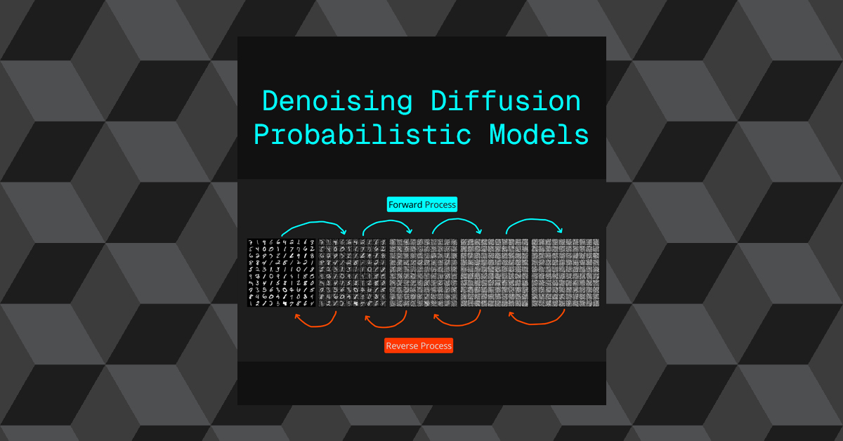
Denoising Diffusion Probabilistic Models (DDPMs) was first introduced in the white paper by Jonathan Ho,Ajay Jain,Pieter Abbeel in 2020. The original academic paper can be found below.
- DDPM academic paper: https://arxiv.org/abs/2006.11239
This academic paper introduces what can be considered the first widely adopted modern diffusion model. Although the diffusion process itself are widely attributed to the paper “Deep Unsupervised Learning using Nonequilibrium Thermodynamics” (Sohl-Dickstein et al., 2015): https://arxiv.org/abs/1503.03585
In this study, I will be focusing on the DDPM academic paper indirectly by breaking down a python implementation of the model along with the math in an effort for me to gain an understanding on how a basic diffusion model produces convincing images.
Below is a visualization of the reverse process, this particular output has been generated by calculating the instantaneous estimation of the final image \(x_0\), calculated at each timestep \(x_{t-1}\) of the reverse process. \(T\) of 1000 has been used. Its worth noting that this is a batch of 100 unique samples (images) being generated.
Please see the section “\(x_0\) Estimation” for more information on the above.
This model has the following properties:
- Diffusion Space: Pixel-space
- Pre-latent model. Resource intensive as a result
- Backbone Architecture: U-Net
- Prediction Type: Noise prediction (ε-prediction)
- Conditioning Type: Unconditional
- Stochasticity: Stochastic (non-deterministic)
- reverse diffusion step samples from a Gaussian and re-injects noise.
Training Examples:
We will be using the MNIST training dataset to keep computation costs down considering this a pixel space diffusion model.
This study will be using the python implementation that was created by Tushar Kumar. The original code can be found in the GitHub link below:
DDPM Overview
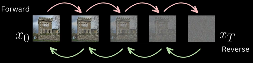
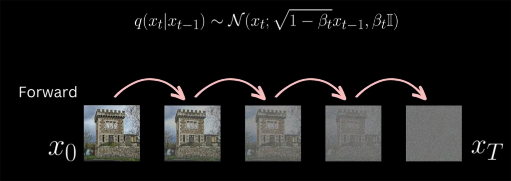
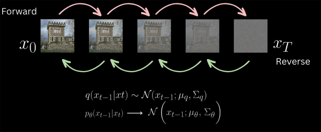
The basic premise of this model is to optimize a neural network to be able to predict noise that has been added to images in varying ratios of signal to noise (signal = image). In the training stage, the model takes images from the training dataset and adds Gaussian noise at different timestep increments, this is referred to as the forward process. The amount of noise that is added to the image increases based on the timestep. At each timestep a U-Net is trained to predict the noise pattern that was added at each incremental timestep. At the final timestep, the image has been completely replaced by noise.
Noise isn’t simply added directly to the original image (signal). Its combined by a ratio that determines how much of the signal gets multiplied down as the noise gets multiplied up before being added together. This ratio increase in favour of the noise as the timesteps increase. For example at \(t=1\) the ratio may be 99% original image (signal) and 1% noise. as \(t\) increases the signal percentage drops and the noise increases.
Once the model has been trained, It will be able to predict the noise in an image at every timestep interval.
If the model has been trained correctly, a novel image known as a sample can be generated by starting from pure Gaussian noise by denoising one timestep at at time backwards until a clean image has been generated, this is know as the reverse process.
The main components of this model are the following:
- Linear Noise Scheduler
- Training: Combines noise with an image, based on the timestep.
- Inference: Subtracts noise from an image, based on the timestep.
- Nueral Network
- U-Net used to generate the predicted noise pattern per timestep.
- Loss Function
- MSE used to calculate the error/loss of each prediction.
- Optomizer
- Adam algorithm used to update parameters within the model, based on the loss function.
Hyperparameters
Below is a breakdown of the hyperparameters that are used in this model, along with their defaults and a brief description.
Diffusion Hyperparameters
These directly control linear noise scheduler, expand below for details.
Diffusion Hyperparameters Details
- num_timesteps: 1000
- Number of forward diffusion steps \(T\)
- The forward process adds noise step by step until the image becomes nearly pure Gaussian noise.
- \(T=1000\) is the default in the original DDPM paper.
- Intuition: more steps → smoother noise schedule and better quality samples, but slower sampling.
- beta_start: 0.0001
- The maximum noise variance \(\beta_0\)
- Controls how little noise is added at the first step. Very small so the model starts with images close to the original.
- beta_end: 0.02
- The maximum noise variance \(\beta_{T-1}\)
- Controls how much noise is added at the final step. Larger than beta_start to ensure near-total corruption at the end.
Together,
beta_start→beta_enddefines a linear noise schedule:\(\beta_t\) =linear interpolation between beta_start and beta_end
This ensures early steps are gentle (retain structure) while later steps overwhelm with noise.
Model Hyperparamters
Model Hyperparameters
These directly control the U-Net model, expand below for details.
Model Hyperparameter Details
- m_channels: 1
1means grayscale (e.g., MNIST). If RGB, this would be3.- The U-Net predicts noise maps of the same shape as the input image.
- im_size: 28
- Image resolution.
- 28 → 28×28
- Important for determining how many down sampling/up sampling steps the U-Net can take.
- down_channels:
- Channel sizes for each level of the U-Net’s down path.
- [32, 64, 128, 256]:
- At input resolution: 32 filters
- After 1st down sample: 64
- After 2nd down sample: 128
- After 3rd down sample: 256
- Intuition: as resolution shrinks, we increase channels to capture richer, more abstract features.
- mid_channels:
- Channel sizes inside the bottleneck (mid blocks).
- [256, 256, 128]: processes the deepest features with residual + attention blocks.
- The last entry (128) matches back to the up path.
- down_sample:
- Whether to apply spatial down sampling at each down block.
[True, True, False]:- 1st down block down samples (H/2, W/2)
- 2nd down block down samples (H/4, W/4)
- 3rd down block keeps resolution constant (no stride)
- Intuition: early down samples increase receptive field; later blocks keep detail.
- time_emb_dim:
- Dimension of the sinusoidal time embedding.
- 128 → each timestep \(t\) is mapped to a 128-D vector
- This vector is injected into ResNet blocks to condition them on the diffusion step.
- num_down_layers:
- Number of ResNet+attention layers inside each DownBlock.
- 2 → each DownBlock repeats [ResNet→Attention] twice.
- Increases representational capacity.
- num_mid_layers:
- Number of [Attention→ResNet] pairs in the MidBlock.
- 2 → deeper processing at the bottleneck.
- num_up_layers:
- Number of ResNet+attention layers inside each UpBlock.
- 2 → each UpBlock mirrors the depth of its DownBlock.
- num_heads:
- Number of heads in multi-head self-attention.
- 4 → each attention layer splits channels into 4 subspaces for parallel attention.
- Helps capture diverse spatial dependencies.
Training Hyperparameters
These directly control the training loop, expand below for details.
Training Hyperparameter Details
- batch_size:
- Number of images per training batch
- 64 → is a standard balance between gradient stability and GPU memory.
- num_epochs:
- How many full passes over the dataset.
- 40 → training continues until all images have been seen 40 times.
- num_samples:
- How many new images to generate during evaluation.
- Typically used to monitor sample quality during training.
- num_grid_rows:
- When saving generated samples as an image grid, how many rows to arrange them into.
- For visualization (e.g., torchvision.utils.make_grid).
- lr:
- Learning rate for optimizer (Adam or AdamW).
- 1e-4 is a common stable choice for DDPMs.
Image Prep
The training set is handled via a class that stores the image paths, each image is converted into a tensor when called upon. The images are expected to have a numerical range between 0-1. The range is offset to be between -1 to 1. This is done to match the gaussian noise range that is added to the image.
Gaussian noise is zero-centred and symmetric.
This is an extract from the class MnistDataset that is responsible for retrieving each image.
    def __getitem__(self, index):
        im = Image.open(self.images[index])
        im_tensor = torchvision.transforms.ToTensor()(im)

        # Convert input to -1 to 1 range.
        im_tensor = (2 * im_tensor) - 1
        return im_tensors
By doing this we are matching the images distribution to the gaussian noise which has a zero centre (mean = 0) and a variance of unit 1 aka -1 to 1 distribution.
To work with high dynamic range images, a number of steps can be taken such as a transform that scales down the range into 0-1 or -1 to 1 or a possibly less stable approach would be to alter the math in the model to deal with the high dynamic range.
No labels are needed because this model is unconditional
Notation
Below represent some of the main elements that will appear throughout.
- \(x_0\) = Clean image from training set
- \(\epsilon\) = Gaussian noise (random tensor, same shape as image).
- \(\epsilon \sim N(0,I)\) = Normal Distribution (Gaussian) zero mean, unit variance
- \(t\) = Timestep
- \(t\in\{1,…,T\}\) (integer, chosen randomly; represents how much noise is applied).
- \(x_t\) = Noisy image at step \(t\), created by gradually mixing \(x_0\) with Gaussian noise.
- \(\hat{\epsilon}_\theta(x_t,t)\) = Predicted noise output by the UNet, conditioned on noisy image \(x_t\) and timestep \(t\) (embedding)
- \(\beta_t\) = Variance schedule at step \(t\) small positive value that controls how much noise is added.
- \(\alpha_t = 1-\beta_t\) Signal preservation factor at step \(t\)
- \(\bar{\alpha_t} = \prod_{s=1}^t\alpha_s\) = Cumulative product of signal preservation up to step \(t\)
Training Pipeline
The logic below applies per image \(x_o\) , however the system works by applying the same logic to a batch of images in parallel at a time. This provides greater efficiencies in both training performance based on the GPU memory but also in providing a more stable gradient direction for optimization.
Along side the explanation, I will be adding code snippets to help illustrate the process.
Linear Noise Schedular
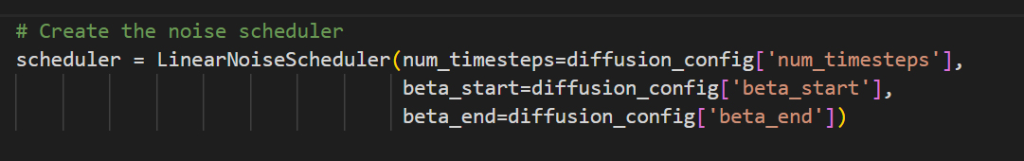
- Initializes the custom noise scheduler to “scheduler”
- scheduler.addNoise() is called in the training loop to apply noise to the original image based on the timestep.
Training Set
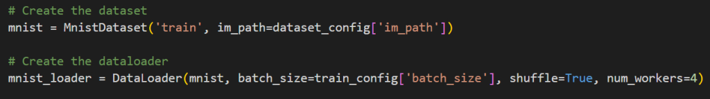
- MnistDataset() is a custom class that converts each image from the training set into a tensor.
- Each image is centered around zero prior to training.
- DataLoader(): Is used to package up the tensor image data in batches , along with shuffling the data in between epoch loops.
U-Net Model
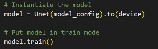
- The custom U-Net model is loaded into the GPU and prepared for training.
- model.train() – Sets internal flags needed for training (Dropout, BatchNorm/LayerNorm, Stochastic behaviour)
The below shows the number of trainable parameters:
    total_params = sum(p.numel() for p in model.parameters() if p.requires_grad)
    print(f"Total trainable parameters: {total_params}")

    ### Total trainable parameters: 10188081
Loss Function & Optomizer
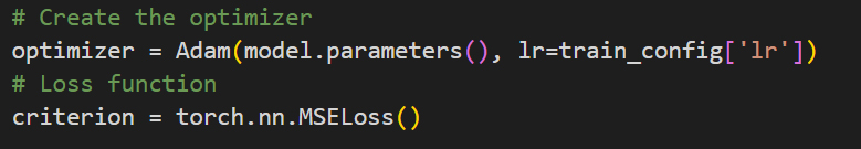
- Adam(): Used to update the each parameter weight based on gradients, learning rate and a update rule.
- MSELoss(): Used to calculate the error rate based on a standard Mean Squared Error function.
Training Loop
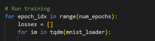
- We loop over each epoch, with each epoch loop, we loop over each batch of images that is pulled from the DataLoader (mnist_loader)
- Steps 1 – 7 occur once per batch per epoch.
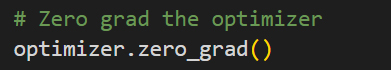
- At the start of each batch loop, any stored gradients are set to zero for every parameter in the optimizer.
- Step 8 occurs at the end of every epoch.
Step 1 – Sample clean image(s)
$$x_0\sim p_{data}(x_0)$$
- Pull a batch of images from the training set.
- Each unit of data that will go through training at a time. This will be referred to as a “batch tensor”.
- \(x_0 \in R^{B\times C\times H\times W}\)
- B = Batch size, C = channels, H = image height, W = image width.
# A single "batch" tensor. Containing 64 images, with 1 channel. Each image is 28x28
torch.Size([64, 1, 28, 28])- For simplicity we will refer to \(x_0\) as a single image within the batch.
- Each \(x_0\) represents the true data distribution that we want the model to learn.
- \(x_0\) is the “ground truth” starting point prior to any noise corruption
- The batch for-loop produces the above mentioned batch tensor , which is sent to the GPU.
- “im” represents the current batch that was produced by the DataLoader
Step 2 – Sample timestep
$$t_i\sim Uniform\{1,…,T\}$$
- Each image in the batch gets its own random timestep \(t_i\)
- This decides how corrupted the image will be (signal vs noise). The model must learn to denoise at all possible corruption levels aka timesteps.
- Intuition: across a batch, some images may be lightly noised, some heavily, giving the network diverse training signals per update.
- torch.randint is used to generate a random integers between zero and \(T\) (max timesteps)
- \(t\) will contain a tensor of random integers. The number of integers will match the batch size.

Step 3 – Sample Gaussian noise
$$\epsilon \sim N(0,I)$$
- Generate random noise tensor with the same shape as \(x_t\)
- Each image gets its own independent Gaussian noise tensor.
- This is the pure Gaussian noise that will be mixed into the \(x_t\) to create \(x_t\)
- randn_like() produces a tensor array of random numbers from a standard normal distribution.
- The tensor stored in “noise” is the same shape as the batch of tensor image data that is fed into randn_like(). Each noise pattern has the same number of channels and resolution as the training images.
Step 4 – Generate noisy image (Forward Process)
$$x_t^{(i)} = \sqrt{\bar{\alpha_t}}x_0^{(i)}+\sqrt{1-\bar{\alpha_t}}\epsilon^{(i)}$$
- Compute noisy images for the whole batch in parallel (using vectorized operation).
- The use of \(i\) in the above formula simply signifies that we apply this formular per image in each batch.
- Signal: \(\sqrt{\bar{\alpha_t}}x_0\) = As t grows, \(\sqrt{\bar{\alpha_t}}\) decreases which is used to multiply down \(x_0\)
- Noise: \(\sqrt{1-\bar{\alpha_t}}\epsilon\) = As t grows, \(\sqrt{1-\bar{\alpha_t}}\) increases which is used to multiply up \(\epsilon \)
- Then the signal and noise is summed together to make \(x_t\)
- The schedular will take the three inputs: “im” original images, “noise” image, “t” random timestep and produce a tensor array that contains a batch of images that have been mixed with noise to various ratios based on the random timestep integer.
Step 5 – Predict noise with U-Net
$$\hat{\epsilon}_\theta(x_t,t)$$
- Feed batch of noisy images \(x_t\) + timesteps embedding of $t$ into the UNet
- Output: predicted noise tensor, same shape as $x_t$. Each image in the batch will get its own noise predictions.
- The model is trying to predict the the exact gaussian pattern that was added to the original image(s). The timestep embedding is used to determine the level of noise that was added and the noise to signal ratio for any particular timestep.
The data distribution of the original image set is learned indirectly from the task of predicting noise. The U-Net needs to identify the different between signal and noise and as a result, it learns the data distribution of the training image set ( signal ). Its the understanding the data distribution of the training set that makes producing samples ( images ) based on the training set possible.
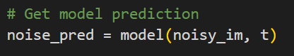
- The custom model uses the “noisy_im” tensor to predict the noise pattern that was used in each image, based on the timestep “t”
- noise_pred” = contains a tensor array of the same shape as “noisy_im”, each tensor image contains the predicted noise pattern that was used in each image.
Step 6 – Compute Loss
$$L(\theta) =\frac{1}{B}\sum_{i=1}^B||\epsilon^{(i)}-\hat{\epsilon_\theta}(x_t^{(i)},t)||^2$$
- Average Mean Square Error (MSE) across the whole batch of individual errors.
- Compare predicted noise \(\hat{\epsilon}\) with the “ground truth” noise \(\epsilon\), per image in the batch
- Here the model calculates loss by subtracting the predicted noise pattern from the real noise pattern that was used to corrupt the original image.
- Intuition: if the model predicts the noise perfectly, subtracting it from the \(x_t\), would recover the clean image \(x_0\)
- Since we are average the loss’s per image, we will refer to this as “batch loss”
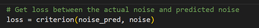
- “criterion” aka MSE is used to calculate the loss by comparing the predicted noise by the original noise.
- the MSELoss() in “criterion” returns the following tensor object:
tensor(0.0134, grad_fn=<MseLossBackward0>)- The float is average squared error across the entire batch.
- Since “grad_fn” is present, the tensor object is part of the computation graph → you can call loss.backward() to compute gradients.
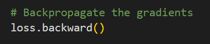
Step 7 – Backpropagation & update weights \(\theta\)
- Backpropagation the batch loss through the network.
- Update all the parameters \(\theta\) (convolution filters, attention weights, etc.) using gradient descent.
- Optimizer (Adam) updates all U-Net weights once per batch.
- Intuition: each update nudges the UNet so it better predicts the true noise. Over many iterations, it becomes a general denoiser for any \(t\)
- A benefit of calculating the loss as an average of the batch of images, we are creating a much more stable gradient direction to update the weights. If we were to update the weights based on a single sample ( one image ), we would get a much more noisy update.
- Let p represent a parameter tensor (all_parameters = model.parameters())
- backward() computes gradients of the loss with respect to all trainable parameters in your model and stores the new gradient value under each parameters “p.grad” tensor attribute. This method does not update the weights, it just calculates and stores the new gradient for each parameter.
- Because the tensor object stored under “loss” has a “grad_fn” attribute, it is connected to the graph. When backward() is executed, PyTorch’s autograd engine walks backward through the computation graph in order to retrieve every trainable parameter within the network.
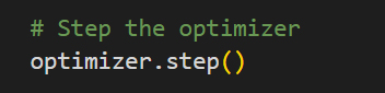
- step() this loops over all parameters tensors (trainable) within the model, reads the “p.grad” gradient data and applies the update rule (SGD,Adam,etc) and then writes the optimized weights into “p.data” for every trainable parameter tensor. Applying the new gradient to .data is what actually updates the weights/biases etc.
- The weights have now be updated with more optimal weights – This whole process is iterated until the error rate is acceptable and the overall weights are considered optimized.
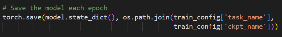
Step 8 – Save tensor checkpoint
- Tensor checkpoint saved out to store the updated weights after every epoch. Most models we use are just states of optimization that are considered usable. Error/Loss is often never 0 in complex systems.
Inference Pipeline
Model
The original model and the optimized weights from training are both loaded.
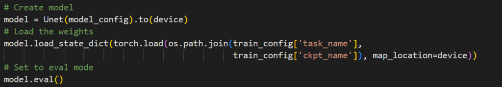
- model.eval() – Sets internal flags needed for inference, ensures deterministic, stable predictions when sampling.
Linear Noise Scheduler
- Initializes the custom noise scheduler to “scheduler”
- scheduler.sample_prev_timestep() is called in the sampling loop to “denoise” the image.
Sampling
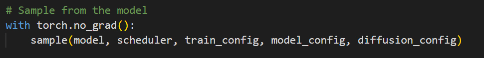
- with torch.no_grad(): This is essential in establishing an optimal state within torch for inference, anything called in the block will operate in this context.
- Autograd does not build a computation graph.
- Tensors created won’t track gradients.
- Saves memory (no .grad_fn, no intermediate storage).
- Speeds up computations (no bookkeeping for backprop).
- Forward Passes only, no learning
Step 1 – Initialize with pure noise
$$x_T \sim N(0,I)$$
- \(x_T\) Represents the noisy image at the maximum timestep \(T\). This is this represents the last timestep that is used in the forward process within the training pipeline.
- The same statistical property of the noise are used, normal distribution, mean = 0 and variances of 1.
- Although not necessary , this sampling process has been set up to infer a batch of samples from the model. This will produce a 100 new images.
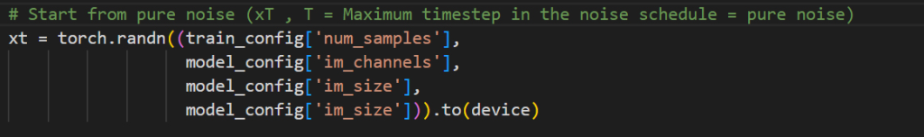
- randn() is used to generate the random noise patterns, the shape of the data matches what was used in the training process.
- xt: shape (B, C, H, W) where B = num_samples.
Step 2 – Reverse Process Loop
- \(x_T\) represents a batch of gaussian noise distributions that represent the last stage of the forward process. We use the reverse process to effectively denoise the image by reversing backwards, one timestep interval at a time. This recursive process eventually resolves into a novel image that has the same data distribution characteristics that was learned in the forward process training phase.
- This loop sets up i to iterate from max timesteps down to zero.
- \(i = t = T,T-1,T-2,T-3,…,0\)

Step 3 – Predict the noise at step t
$$\hat{\epsilon}=\hat{\epsilon}_\theta(x_t,t)$$
- The U-Net model that was trained to predict noise in the training phase, is now used to predict the noise again. This time we are starting from pure noise and stepping backwards based on the one timestep at a time.
- This predicted noise will be used to denoise the image \(x_T\). The process is designed to follow the same logic as the forward process, but in reverse. So at each timestep, we are only interested in denoising the image by the amount of noise that was added for the given timestep.

Step 4 – Reverse Noise Step
- This step is where the initial pure noise image is “denoised” by a single timestep.
- The noise prediction that was produced by the model \(\hat{\epsilon}\) along with the current timestep \(t\) is used to calculate the previous timestep state.
- when i = \(T\) , this step will calculate what \(x_T\) would be when i = \(T-1\), the previous timestep in the reverse process.
- The scheduler uses:
- xt = The batch of noisy images , initially starting from pure noise.
- noise_pred = the noise that has been predicted from the current timestep
- i = which represents \(t\) , starting from \(T\), then sequentially revering down to 0 (\(T-1,T-2,T-3,…0\))

- sample_prev_timestep(): outputs two different batches of images.
- xt: This is the batch of noisy images that have had the current time steps noise removed. If the current timestep was 10 for example , this is what the image would be at $t=9$. When the loop goes through its next iteration xt will become what the noisy images look like at \(t=8\) and so on.
- xt: on the next iteration of the loop, this data is feed back into the model to recalculate the predicted noise, which is then used to step back another step, incrementally denoising the original pure noise back into fully formed image.
- x0_pred: This optionally can be used to see what the estimated clean image would be: \(\hat{x_0}\)
Denoising
In order to understand how the denoising works we will dive further into the linear noise scheduler, specifically the scheduler.sample_prev_timestep() method.
Function Pre-requisites
Betas \(\beta_t\)

- \(\beta_t \in R^T\) : betas = evenly spaced between beta_start and beta_end
- Shape: (T,)
Alphas \(\alpha_t\)
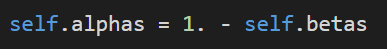
- \(\alpha_t = 1 – \beta_t\)
- Shape: (T,)
Alphas Cumulative Product \(\bar{a}_t \)

- \(\bar{a}_t = \prod_{s=0}^t\alpha_s\)
- How much signal remains after \(t\) forward-noise steps
- Shape: (T,)
Square Root Cumulative Products

- \(\sqrt{\bar{\alpha_t}}\) and \(\sqrt{1-\bar{\alpha_t}}\) precomputed.
Reverse Noise Step
This video visualizes the exact state of the image being denoised through the reverse process all the way from \(x_T\) (pure Gaussian noise) down to \(x_0\) (clean image). \(T\) of 1000 has been used. Its worth noting that this is a batch off 100 unique samples (images) being generated.

- Inputs:
xt= current noisy state \(x_t\) , Shape (B,C,H,W)noise_pred= \(\hat{\epsilon}(x_t,t)\) ,Shape (B,C,H,W)t= scalar timestep (shared across batch during sampling)
Compute reverse mean / Posterior Mean \(\mu_t\)
$$\mu_t(x_t,\hat{\epsilon}) = \frac{1}{\sqrt{\alpha_t}}\huge(\normalsize x_t-\frac{\beta_t}{\sqrt{1-\bar{\alpha_t}}}\hat{\epsilon}(x_t,t)\huge)$$

- First line calculates within the brackets
- \(x_t-\frac{\beta_t}{\sqrt{1-\bar{\alpha_t}}}\hat{\epsilon}(x_t,t)\)

- Second line handles the coefficient by using division instead of multiplying, as the numerator is 1, we simply divide by the square root.
- \(\frac{1}{\sqrt{\alpha_t}}\)
- mean=\(\mu_t\)
Add Calibrated Noise
Noise is re-added at each step , with the exception of \(t\) =0, as the image is considered clean and requires no further denoising as this stage.
$$x_{t-1}= \large\begin{cases} \normalsize \mu_t, &\normalsize \text{if } t=0 \\ \normalsize \mu_t +\sigma _tz, \ z \sim N(0,I) &\normalsize\text{else } t>0 \end{cases}$$
- Noise reintroduction keeps the reverse process a stochastic Markov chain that correctly models the forward process distribution.
- if t = 0:
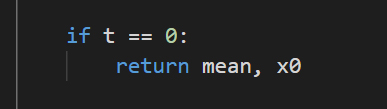
- When at the end of the reverse process we simply return the posterior mean , without re-adding noise.
- t > 0:
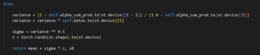
- When at a intermediary step of the reverse process we re-add noise back into the posterior mean

- \(\bar \beta_t\) = Posterior Variance
$$\bar{\beta}_t = \frac{1-\bar{\alpha_t}_{-1}}{1-\bar{\alpha}_t}\beta_t%%
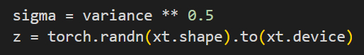
- \(\sigma (sigma)\) = square root of \(\bar \beta_t\)
- \(\sigma = \sqrt{\bar{\beta_t}}\)
- z =noise = \(z \sim N(0,I)\) (same shape as xt).
- The noise / variance is used to add calibrated stochasticity back (diversity; probabilistic correctness).

- Returns the predicted image at \(x_{t-1}\) (mean) while adding noise multiplied by variance
- \(x_{t-1} = \mu_t +\sigma _tz\)
\(x_0\) Estimation
- In addition to the reverse process being used to iteratively deduct predicted noise until we reach our clean image \(x_0\).
- This function also predicts a instantaneous clean image \(x_0\), this is achieved by algebraically inverting the forward equation to be able to estimate \(x_0\) at any timestep interval \(t\)
$$\hat{x}_0 \frac{x_t – \sqrt{1-\bar{\alpha}_t\hat{\epsilon}}}{\sqrt{\bar{\alpha}_t}}$$

- self.sqrt_one_minus_alpha_cum_prod[t]
is \(\sqrt{1-\bar{\alpha}_t}\) - torch.sqrt(self.alpha_cum_prod[t])
is \(\sqrt{\bar{\alpha}_t}\) - Broadcasted across (B,C,H,W).
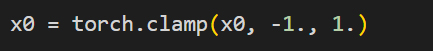
- keep \(\hat x\) in the training data range [-1,1] for stability and realism
- Through out the above code, x0
Step 5 – Post-Processing
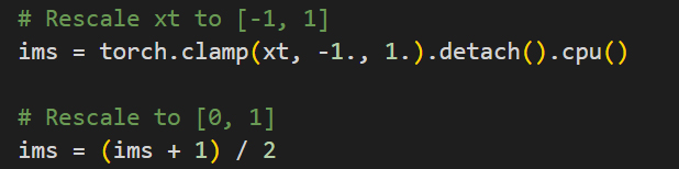
The current timestep gets saved out, this represents the current state of the image \(x_t\).
Before doing so, the the image is transformed back into a 0-1 distribution.

Step 6 – Repeat loop until we have a clean image
Until the reverse process reaches 0, the loop will take the output from the current iteration and feed that back into the next iteration, which will iteratively denoise the \(x_t\) until we get to \(x_0\) which is a clean image.